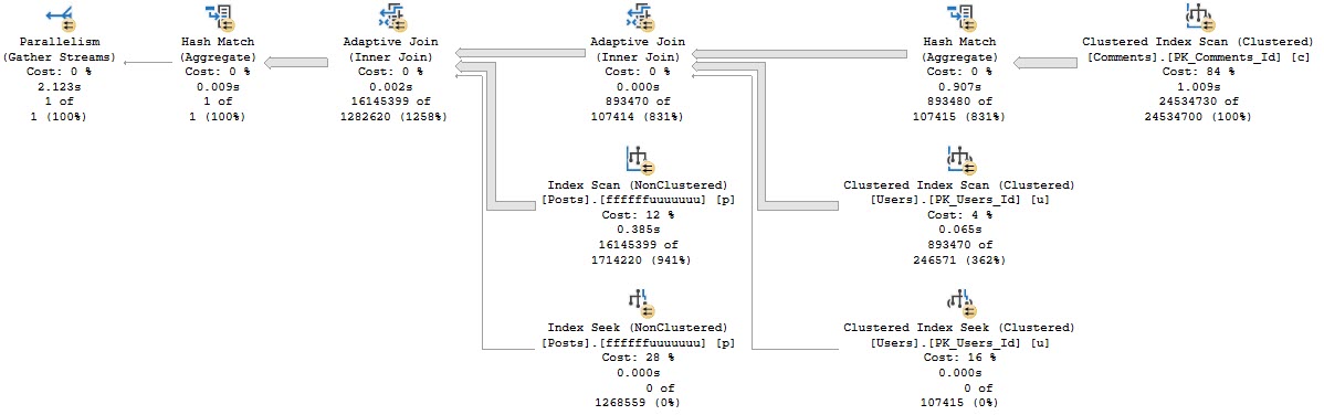
SQL Server friend and excellent webmaster Mr. Erik C. Darling showed me a query plan gone wrong:
 48 billion rows for a single operator is certainly a large number for most workloads. I ended up completely missing the point and started wondering how quickly a query could process a trillion rows through a single operator. Eventually that led to a SQL performance challenge: what is the fastest that you can get an actual plan with at least one operator processing a trillion rows? The following rules are in play:
- Start with no user databases
- Any query can run up to MAXDOP 8
- Temp tables may be created and populated but all such work needs to finish in 30 seconds or less
- A RECOMPILE query hint must be present in the final query
- Undocumented features and behavior are fair game
Unless stated otherwise here, all testing was done on SQL Server 2017 CU20. The processor of my local machine is an Intel i7-9700K. If you’re following along at home you may see different results depending on your hardware. The queries are extremely CPU intensive. If you’d like to skip ahead to the winning query then scroll down the bottom.
Loop Join
A natural way to generate a lot of rows quickly is to cross join together two equally sized tables. Throwing a million rows into a temporary table takes very little time. Finding the count of the result set should meet the challenge requirements as long as the right optimizer transforms are not available. An initial attempt for data prep:
DROP TABLE IF EXISTS #loop_test;

CREATE TABLE #loop_test (
ID TINYINT NOT NULL
);

INSERT INTO #loop_test WITH (TABLOCK)
SELECT TOP (1000000) CAST(0 AS TINYINT) ID
FROM master..spt_values t1
CROSS JOIN master..spt_values t2
OPTION (MAXDOP 1);

CREATE STATISTICS S1 ON #loop_test (ID) WITH FULLSCAN, NORECOMPUTE;
Along with the query to run:
SELECT COUNT_BIG(*)
FROM #loop_test t1 WITH (TABLOCK)
CROSS JOIN #loop_test t2 WITH (TABLOCK)
OPTION (RECOMPILE, MAXDOP 8);
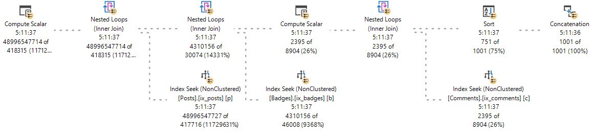
The query returns the expected result of 1 trillion, but there is no operator that processes one trillion rows:
The query optimizer uses the LocalAggBelowJoin rule to perform an aggregate before the join. This brings down the total query estimated cost from 1295100 units to 6.23274 units for quite a savings. Trying again after disabling the transform:
SELECT COUNT_BIG(*)
FROM #loop_test t1 WITH (TABLOCK)
CROSS JOIN #loop_test t2 WITH (TABLOCK)
OPTION (RECOMPILE, MAXDOP 8, QueryRuleOff LocalAggBelowJoin);
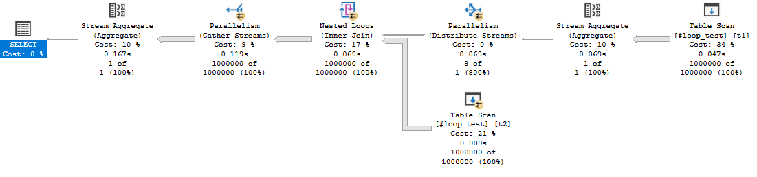
Results in a new query plan:
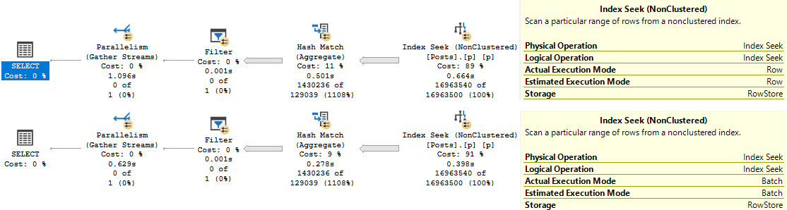
This query meets the requirements of the challenge. The stream aggregate, nested loops, and row count spool operators will process 1 trillion rows each. However, it is unsatisfactory from a performance point of view. The row mode stream aggregate has a significant profiling penalty compared to a batch mode hash aggregate alternative. It is simple enough to create a dummy table to add batch mode eligibility for the query plan:
DROP TABLE IF EXISTS #cci;
CREATE TABLE #cci (ID INT, INDEX CCI CLUSTERED COLUMNSTORE)

SELECT COUNT_BIG(*)
FROM #loop_test t1 WITH (TABLOCK)
CROSS JOIN #loop_test t2 WITH (TABLOCK)
LEFT OUTER JOIN #cci ON 1 = 0
OPTION (RECOMPILE, MAXDOP 8, QueryRuleOff LocalAggBelowJoin);
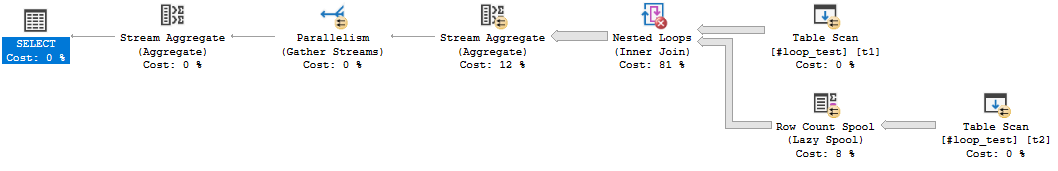
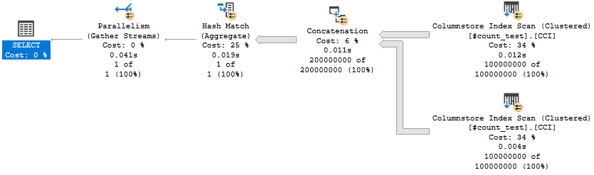
The new plan has a nice batch mode operator to do the counting:
With an actual plan request, the new query processes rows at roughly twice the rate as the row mode query. Perhaps query profiling does its work once per batch for batch mode operators and once per row for row mode operators. Each batch has around 900 rows so profiling might be much cheaper per row for the hash aggregate compared to the stream aggregate. Strictly speaking, the goal of this challenge is to optimize the amount of time it takes to get an actual plan. This might lead to different tuning results than optimizing for query completion time without an actual plan request.
The final time for the batch mode query is 2 hours and 12 minutes. I uploaded an actual plan to pastetheplan.com. The query has a CPU to elapsed time ratio of only 5.37. That means on that average during query execution, more than 2.5 CPU cores were not doing useful work. Getting all eight CPU cores to perform work as much as possible during query execution should allow the query to finish faster. The CPU imbalance in this case is caused by how rows are distributed to threads on the outer side of the nested loop operator:
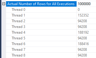
The query engine has different algorithm choices to perform a parallel scan of a table. In this case, it doesn’t pick an algorithm that leads to optimal performance. The nested loop operator in total drives 42717 seconds of CPU work. It’s important to have that work as balanced between threads as possible. In this situation it is helpful to reduce the number of rows per page. To understand why I recommend watching this Pass Summit presentation by Adam Machanic. This results in better row distribution between threads and theoretically better performance. The following code only allows for a single row per data page:
DROP TABLE IF EXISTS #wide_1_million_rows;

CREATE TABLE #wide_1_million_rows (
ID TINYINT NOT NULL,
FILLER VARCHAR(4200) NOT NULL
);

INSERT INTO #wide_1_million_rows WITH (TABLOCK)
SELECT TOP (1000000) CAST(0 AS TINYINT) ID, REPLICATE('Z', 4200) FILLER
FROM master..spt_values t1
CROSS JOIN master..spt_values t2
OPTION (MAXDOP 1);

CREATE STATISTICS S1 ON #wide_1_million_rows (ID) WITH FULLSCAN, NORECOMPUTE;
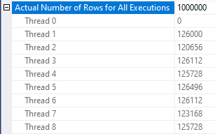
The new query plan generates in 1:29:40 with a CPU ratio of the query is 7.977 which is near perfect. Rows are quite balanced between threads:
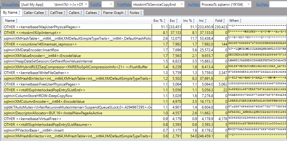
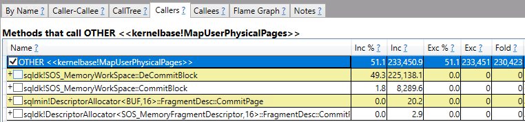
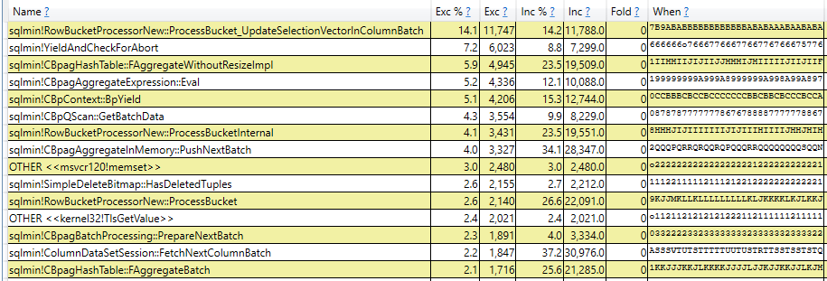
I don’t know of a method to further optimize the nested loop join query. Most of the query’s execution time is spent on profiling. Sampled stacks from 15 seconds of query execution:
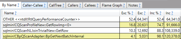
ETW tracing tools such as PerfView along with internals knowledge can be used to more finely break down how CPU is used by this query. Almost 75% of the query’s execution time is spent on sqlmin!CQScanProfileNew:GetRowImp and on methods called by it. The query only takes 23 minutes to complete without an actual plan which is quite close to 25% of the runtime with an actual plan. If you’re interested in more examples of using PerfView to draw conclusiosn about SQL Server consider checking out the list of links in this stack exchange answer.
Merge Join
A cross join can only be implemented as a nested loop join but the same end result can be emulated with a merge join. Let’s start with testing a MAXDOP 1 query. Setup:
DROP TABLE IF EXISTS #cci;
CREATE TABLE #cci (ID INT, INDEX CCI CLUSTERED COLUMNSTORE)

DROP TABLE IF EXISTS #merge_serial;

CREATE TABLE #merge_serial (
ID TINYINT NOT NULL
);

INSERT INTO #merge_serial WITH (TABLOCK)
SELECT TOP (1000000) 0 ID
FROM master..spt_values t1
CROSS JOIN master..spt_values t2
OPTION (MAXDOP 1);

CREATE CLUSTERED INDEX CI ON #merge_serial (ID);
The query to run:
SELECT COUNT_BIG(*)
FROM #merge_serial t1 WITH (TABLOCK)
INNER JOIN #merge_serial t2 WITH (TABLOCK) ON t1.ID = t2.ID
LEFT OUTER JOIN #cci ON 1 = 0
OPTION (RECOMPILE, MERGE JOIN, MAXDOP 1, QueryRuleOff LocalAggBelowJoin);
I did not allow the query to run to completion because it would have taken around 25 hours to complete. On an 8 core machine with merge join, there’s no reason to expect that a parallel query could do any better than 25/8 = 3.125 hours. This makes merge join an inferior option compared to loop join so there isn’t a good reason to pursue further approaches that use a merge join.
For completeness, the best merge plan time I was able to get was 5 hours and 20 minutes. The plan avoids the scalability issues found with parallel merge and order preserving repartition streams. The end result is still poor. The merge join simply consumes a lot of CPU to do its work. The additional overhead added by the loop join is not helpful.
Row Mode Hash Join
Perhaps we’ll have more luck with a hash join compared to a merge join. After all, the query optimizer assigns a lower estimated cost for a row mode hash join compared to a merge join for the trillion row scenario. What could go wrong? The first thing that goes wrong is that the addition of the empty CCI will lead to a batch mode hash join for this query. Avoiding that requires changing the join to a type that doesn’t allow for batch mode execution. Among other methods, this can be accomplished by putting the hash join on the inner side of a nested loop or changing the join to also match on NULL. The second technique will be used at first because it leads to significantly less overhead compared to the loop join approach.
Starting again with a MAXDOP 1 test:
DROP TABLE IF EXISTS #cci;
CREATE TABLE #cci (ID INT, INDEX CCI CLUSTERED COLUMNSTORE)

DROP TABLE IF EXISTS #hash_maxdop_1;
CREATE TABLE #hash_maxdop_1 (
	ID TINYINT NULL
);

INSERT INTO #hash_maxdop_1 WITH (TABLOCK)
SELECT TOP (1000000) 0
FROM master..spt_values t1
CROSS JOIN master..spt_values t2
OPTION (MAXDOP 1);

CREATE STATISTICS S1 ON #hash_maxdop_1 (ID) WITH FULLSCAN, NORECOMPUTE;
The test query has a more complex join condition:
SELECT COUNT_BIG(*)
FROM #hash_maxdop_1 t1 WITH (TABLOCK)
INNER HASH JOIN #hash_maxdop_1 t2 WITH (TABLOCK) ON t1.ID = t2.ID OR (t1.ID IS NULL AND t2.ID IS NULL)
LEFT OUTER JOIN #cci ON 1 = 0
OPTION (MAXDOP 1, RECOMPILE)
Note how the join now includes rows where both sides are NULL. There are no such rows in the table but the query optimizer does not know that so a row mode join is used. The query completed in 5.5 hours. This means that a parallel hash join approach could be competitive with the nested loop join. An optimistic time estimate for a parallel query is 41 minutes.
Getting a parallel query isn’t as simple as changing MAXDOP from 1 to 8 will not have the desired effect. Take a look at the following query plan born from such an attempt:
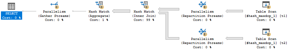
The repartition stream operators have a partitioning type of hash. That means that a hashing algorithm is used to assign rows to different threads. All of the rows from the table have the same column value, so they will all hash to the same value and will end up on the same thread. Seven CPUs will have no work to do even though the query technically executes at DOP 8. This will not lead to performance that’s better than executing at DOP 1.
Through testing I found that the following values for a nullable TINYINT all go to different threads: 0, 1, 4, 5, 7, 9, 14, and 17. Note that I’m relying on undocumented details here that might change between releases. Inserting 250k rows of each value into one table and 500k rows of each value into another table should result in 8 * 250000 * 500000 = 1 trillion rows total. Code to do this is below:
DROP TABLE IF EXISTS #cci;
CREATE TABLE #cci (ID INT, INDEX CCI CLUSTERED COLUMNSTORE)

DROP TABLE IF EXISTS #row_hash_join_repartition_8_build;
CREATE TABLE #row_hash_join_repartition_8_build (
	ID TINYINT NULL
);

INSERT INTO #row_hash_join_repartition_8_build
SELECT TOP (2000000) CASE ROW_NUMBER() OVER (ORDER BY (SELECT NULL)) % 8
WHEN 0 THEN 0
WHEN 1 THEN 1
WHEN 2 THEN 4
WHEN 3 THEN 5
WHEN 4 THEN 7
WHEN 5 THEN 9
WHEN 6 THEN 14
ELSE 17
END
FROM master..spt_values t1
CROSS JOIN master..spt_values t2
OPTION (MAXDOP 1);

CREATE STATISTICS S1 ON #row_hash_join_repartition_8_build (ID) WITH FULLSCAN, NORECOMPUTE;


DROP TABLE IF EXISTS #row_hash_join_repartition_8_probe;
CREATE TABLE #row_hash_join_repartition_8_probe (
	ID TINYINT NULL
);

INSERT INTO #row_hash_join_repartition_8_probe
SELECT TOP (4000000) CASE ROW_NUMBER() OVER (ORDER BY (SELECT NULL)) % 8
WHEN 0 THEN 0
WHEN 1 THEN 1
WHEN 2 THEN 4
WHEN 3 THEN 5
WHEN 4 THEN 7
WHEN 5 THEN 9
WHEN 6 THEN 14
ELSE 17
END
FROM master..spt_values t1
CROSS JOIN master..spt_values t2
CROSS JOIN master..spt_values t3
OPTION (MAXDOP 1);

CREATE STATISTICS S1 ON #row_hash_join_repartition_8_probe (ID) WITH FULLSCAN, NORECOMPUTE;
Along with the query to run:
SELECT COUNT_BIG(*)
FROM #row_hash_join_repartition_8_build t1 WITH (TABLOCK)
INNER JOIN #row_hash_join_repartition_8_probe t2 WITH (TABLOCK) ON t1.ID = t2.ID OR (t1.ID IS NULL AND t2.ID IS NULL)
LEFT OUTER JOIN #cci ON 1 = 0
OPTION (RECOMPILE, HASH JOIN, MAXDOP 8, QueryRuleOff LocalAggBelowJoin);
The query plan appeared after 42 minutes with a CPU ratio of 7.7. This was a better result than I was expecting. The repartition stream operators don’t seem to have much of a negative effect on overall runtime.
For completeness, I also tested a parallel hash join plan without the repartition stream operators. All of the hash join work is on the inner side of a nested loop join. The loop join adds significant overhead so this ends up being a losing method. If you’d like to see for yourself, here is one way to set up the needed tables:
DROP TABLE IF EXISTS #cci;
CREATE TABLE #cci (ID INT, INDEX CCI CLUSTERED COLUMNSTORE)

DROP TABLE IF EXISTS #hash_join_demand_62500_rows;
CREATE TABLE #hash_join_demand_62500_rows (
	ID TINYINT NOT NULL
);

INSERT INTO #hash_join_demand_62500_rows WITH (TABLOCK)
SELECT TOP (62500) ISNULL(CAST(0 AS TINYINT), 0) ID
FROM master..spt_values t1
CROSS JOIN master..spt_values t2
OPTION (MAXDOP 1);

CREATE STATISTICS S1 ON #hash_join_demand_62500_rows (ID);
As well as one way to generate such a query:
SELECT COUNT_BIG(*)
FROM
(VALUES
	  (0),(0),(0),(0),(0),(0),(0),(0)
	, (0),(0),(0),(0),(0),(0),(0),(0)
	, (0),(0),(0),(0),(0),(0),(0),(0)
	, (0),(0),(0),(0),(0),(0),(0),(0)
	, (0),(0),(0),(0),(0),(0),(0),(0)
	, (0),(0),(0),(0),(0),(0),(0),(0)
	, (0),(0),(0),(0),(0),(0),(0),(0)
	, (0),(0),(0),(0),(0),(0),(0),(0)
	, (0),(0),(0),(0),(0),(0),(0),(0)
	, (0),(0),(0),(0),(0),(0),(0),(0)
	, (0),(0),(0),(0),(0),(0),(0),(0)
	, (0),(0),(0),(0),(0),(0),(0),(0)
	, (0),(0),(0),(0),(0),(0),(0),(0)
	, (0),(0),(0),(0),(0),(0),(0),(0)
	, (0),(0),(0),(0),(0),(0),(0),(0)
	, (0),(0),(0),(0),(0),(0),(0),(0)
	, (0),(0),(0),(0),(0),(0),(0),(0)
	, (0),(0),(0),(0),(0),(0),(0),(0)
	, (0),(0),(0),(0),(0),(0),(0),(0)
	, (0),(0),(0),(0),(0),(0),(0),(0)
	, (0),(0),(0),(0),(0),(0),(0),(0)
	, (0),(0),(0),(0),(0),(0),(0),(0)
	, (0),(0),(0),(0),(0),(0),(0),(0)
	, (0),(0),(0),(0),(0),(0),(0),(0)
	, (0),(0),(0),(0),(0),(0),(0),(0)
	, (0),(0),(0),(0),(0),(0),(0),(0)
	, (0),(0),(0),(0),(0),(0),(0),(0)
	, (0),(0),(0),(0),(0),(0),(0),(0)
	, (0),(0),(0),(0),(0),(0),(0),(0)
	, (0),(0),(0),(0),(0),(0),(0),(0)
	, (0),(0),(0),(0),(0),(0),(0),(0)
	, (0),(0),(0),(0),(0),(0),(0),(0)
) v(v)
CROSS JOIN (
	SELECT 1 c
	FROM #hash_join_demand_62500_rows t1 WITH (TABLOCK)
	INNER HASH JOIN #hash_join_demand_62500_rows t2 WITH (TABLOCK) ON t1.ID = t2.ID
) ca
LEFT OUTER JOIN #cci ON 1 = 0
OPTION (RECOMPILE, FORCE ORDER, MAXDOP 8, MIN_GRANT_PERCENT = 99, NO_PERFORMANCE_SPOOL);
It might be difficult to understand what’s going on here, so here’s a picture of the query plan:
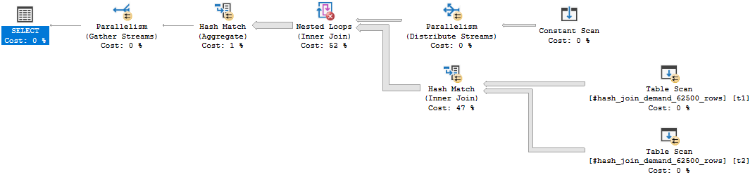
Work is split up into 256 buckets. Each row fed into the outer side of the nested loop join results in 62500 rows hash joined with 62500 rows.
The disappointing final result takes about 2 hours of runtime. This query might perform better on a busy system compared to the simple parallel hash join because work is assigned to threads somewhat on demand. In this case, the repartition streams query query requires equal work to be completed on all threads. However, the testing environment only has a single query running at a time.
The query pattern here is similar to a parallel apply. Perhaps you’ve heard good things about that pattern and are wondering why it didn’t work out here. In my experience, that query pattern does best when an order preserving repartition streams operator can be avoided, there’s a supporting index on the inner side, and the row count coming out of the inner side is relatively low. The above query is 0 for 3.
Batch Mode Hash Join
I’ll be honest. I expected batch mode hash join to be the winner. I was wrong. Batch mode parallelism works in a fundamentally different way than row mode parallelism. There is no repartition streams operator which assigns rows to different threads based on a hash or other algorithm. Rather, each operator takes care of parallelism by itself. In my experience this is generally quite advantageous for both performance and scalability, but there can be drawbacks.
We intend to get a batch mode hash join, so it seems logical enough to join together a CCI with one million rows. Sample code to do that:
DROP TABLE IF EXISTS #batch_mode_hash_equal_sized;

CREATE TABLE #batch_mode_hash_equal_sized (
ID TINYINT NOT NULL,
INDEX CCI CLUSTERED COLUMNSTORE
);

INSERT INTO #batch_mode_hash_equal_sized WITH (TABLOCK)
SELECT TOP (1000000) CAST(0 AS TINYINT) ID
FROM master..spt_values t1
CROSS JOIN master..spt_values t2
OPTION (MAXDOP 1);

CREATE STATISTICS S1 ON #batch_mode_hash_equal_sized (ID) WITH FULLSCAN, NORECOMPUTE;
The query to be run no longer needs the join to the empty CCI table:
SELECT COUNT_BIG(*)
FROM #batch_mode_hash_equal_sized c1
INNER JOIN #batch_mode_hash_equal_sized c2 ON c1.ID = c2.ID
OPTION (RECOMPILE, MAXDOP 8, QueryRuleOff LocalAggBelowJoin);
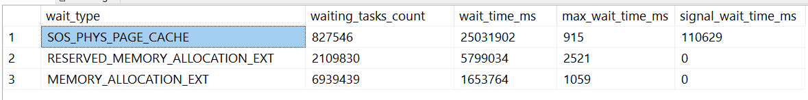
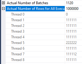
An actual plan is generated on my machine in about 27.5 minutes. While clearly better than all other attempts so far, the CPU to elapsed ratio suggests that significant improvement is possible: it is only 4.6 out of a possible 8.0. Batch mode processing is generous enough to provide a helpful wait stat. There is about 5607 seconds of the HTDELETE wait. Put simply, some of the threads of the hash join ran out of work to do and waited for the other threads to finish their work. As I understand it with batch mode joins, the probe side is what matters in terms of work imbalance. Row count per thread of the probe side:
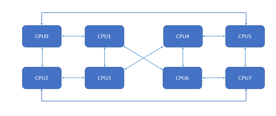
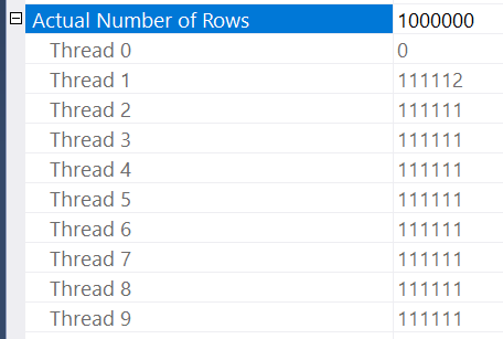
The million row CCI table is split up into 9 chunks of rows which are divided between 8 threads which leads to many threads having no work to do for a while. Quite unfortunate. Oddly enough, switching to MAXDOP 9 could lead to much better performance for this query. That isn’t an available option on my local machine so I switched to testing on a VM with Intel 8280 sockets. The theory works out: the MAXDOP 8 query takes 50 minutes to complete and the MAXDOP 9 query takes 25 minutes to complete. At MAXDOP 9 the row distribution is quite nice on the probe side:
The rules for the different algorithms available to do parallel scans on CCIs are not documented. I previously investigated it here. Interestingly enough, this is an example where an exchange operator could make a positive difference. However, the batch mode hash join doesn’t have that as an option. While there are various tricks to achieve even row distribution from a CCI, it seems simplest to just replace the tables with row store. Converting 2 million rows from row mode to batch mode won’t add any measurable overhead. Using the same table that was used for the best loop join time:
SELECT COUNT_BIG(*)
FROM #wide_1_million_rows c1
INNER JOIN #wide_1_million_rows c2 ON c1.ID = c2.ID
LEFT OUTER JOIN #cci ON 1 = 0
OPTION (RECOMPILE, MAXDOP 8, QueryRuleOff LocalAggBelowJoin)
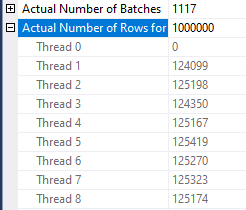
The new query plan finishes in just under 16 minutes. Row distribution per thread on the probe side is much more even:
You might be thinking that 16 minutes is a pretty good result. I too initially thought that.
The Winner
All of the previous approaches spent the vast majority of their time performing a join to generate rows from smaller tables. The scans of the underlying tables themselves were quite fast. Perhaps a better approach would be to avoid the join entirely. For example, consider inserting a billion rows into a table and scanning that table 1000 times with UNION ALL. That would send one trillion rows to a single operator without the expense of a join. Of course, the downside is that SQL Server would need to read one trillion rows total from a table. It would be important to make the reading of rows as efficient as possible. The most efficient method I know is to create a columnstore table with extreme compression.
The title of this section gives it away, but let’s start with a small scale test to see if the approach has merit. Code to load 100 million rows into a CCI:
DROP TABLE IF EXISTS #count_test;

CREATE TABLE #count_test (
ID TINYINT NOT NULL,
INDEX CCI CLUSTERED COLUMNSTORE
);

INSERT INTO #count_test WITH (TABLOCK)
SELECT TOP (100000000) 0 ID
FROM master..spt_values t1
CROSS JOIN master..spt_values t2
CROSS JOIN master..spt_values t3
OPTION (MAXDOP 1);

CREATE STATISTICS S1 ON #count_test (ID);
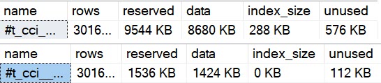
SQL Server is able to compress this data quite well because there’s just a single unique value. The table is only 1280 KB in size. The data prep code does exceeds the 30 second time limit on my machine due to the statistics creation, but I’ll ignore that for now because it’s just a trial run. I can avoid all types of early aggregation with the following syntax:
SELECT COUNT_BIG(*)
FROM
(
	SELECT ID
	FROM #count_test
	UNION ALL
	SELECT ID
	FROM #count_test
) q
OPTION (RECOMPILE, MAXDOP 8, FORCE ORDER)
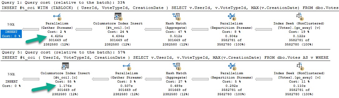
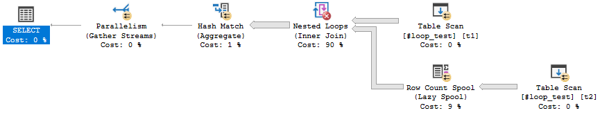
Picture of the query plan:
On my machine, that query takes about 41 ms to process 200 million rows. Based on that, it seems reasonable to expect that a query that processes a trillion rows could finish in under four minutes. There is a balancing act to perform here. Putting more rows into the table makes it harder to complete data prep within 30 seconds, but cuts down on the number of UNION ALLs performed which reduces query compilation time.
The approach that I settled on was to load 312.5 million rows into a table. Reading that table 3200 times results in a trillion total rows. 3200 is a convenient number to achieve with nested CTEs and I’m able to load 312.5 million rows quite reliably under 30 seconds even with MAXDOP 4. I can’t say that this is the best possible approach but it seems to work fairly well.
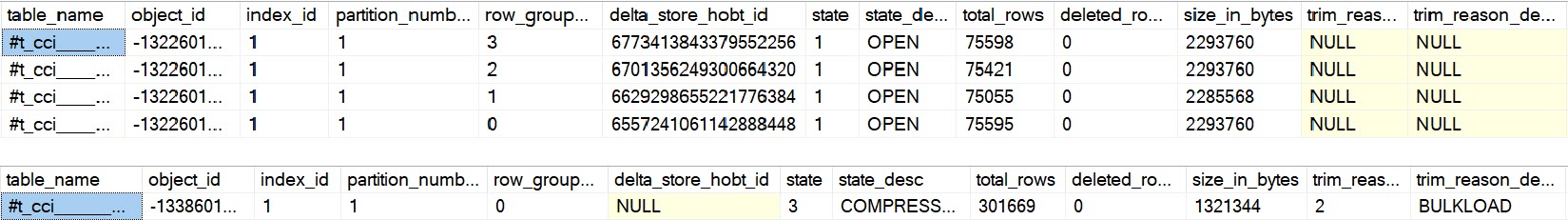
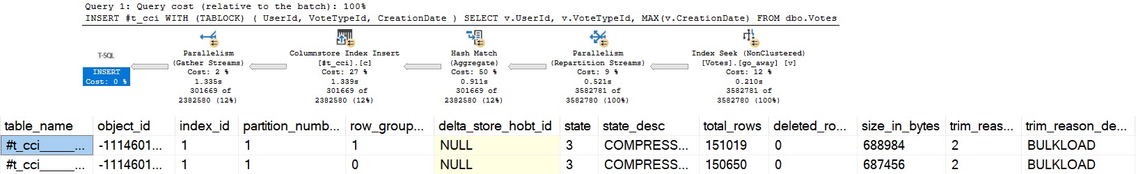
The last detail in terms of data prep is to deal with statistics creation. SQL Server forces a sample rate of 100% for very small tables. Unfortunately, extremely compressed columnstore indexes can fall into the 100% range even if they have a high row count. Creating a statistic object with a sample of 312.5 million rows will take longer than 30 seconds. I don’t need good statistics for query performance so I work around the issue by creating a statistic with NORECOMPUTE after an initial load of 500k rows. Code to create and populate a CCI with 312.5 million rows:
DROP TABLE IF EXISTS #CCI_1M_ONE_COLUMN;

CREATE TABLE #CCI_1M_ONE_COLUMN (ID TINYINT NOT NULL, INDEX I CLUSTERED COLUMNSTORE);

DECLARE @insert_count TINYINT = 0;
WHILE @insert_count < 8
BEGIN
	INSERT INTO #CCI_1M_ONE_COLUMN
	SELECT TOP (125000) 0
	FROM master..spt_values t1
	CROSS JOIN master..spt_values t2
	OPTION (MAXDOP 1);

	SET @insert_count = @insert_count + 1;
END;

DROP TABLE IF EXISTS #C;

CREATE TABLE #C (I TINYINT NOT NULL, INDEX I CLUSTERED COLUMNSTORE);

INSERT INTO #C WITH (TABLOCK)
SELECT TOP (500000) 0
FROM #CCI_1M_ONE_COLUMN
OPTION (MAXDOP 1);

CREATE STATISTICS S ON #C (I) WITH NORECOMPUTE, FULLSCAN;

WITH C13 AS (
	SELECT ID FROM #CCI_1M_ONE_COLUMN
	UNION ALL
	SELECT ID FROM #CCI_1M_ONE_COLUMN
	UNION ALL
	SELECT ID FROM #CCI_1M_ONE_COLUMN
	UNION ALL
	SELECT ID FROM #CCI_1M_ONE_COLUMN
	UNION ALL
	SELECT ID FROM #CCI_1M_ONE_COLUMN
	UNION ALL
	SELECT ID FROM #CCI_1M_ONE_COLUMN
	UNION ALL
	SELECT ID FROM #CCI_1M_ONE_COLUMN
	UNION ALL
	SELECT ID FROM #CCI_1M_ONE_COLUMN
	UNION ALL
	SELECT ID FROM #CCI_1M_ONE_COLUMN
	UNION ALL
	SELECT ID FROM #CCI_1M_ONE_COLUMN
	UNION ALL
	SELECT ID FROM #CCI_1M_ONE_COLUMN
	UNION ALL
	SELECT ID FROM #CCI_1M_ONE_COLUMN
	UNION ALL
	SELECT ID FROM #CCI_1M_ONE_COLUMN
)
, C312 AS
 (
	SELECT ID FROM C13
	UNION ALL
	SELECT ID FROM C13
	UNION ALL
	SELECT ID FROM C13
	UNION ALL
	SELECT ID FROM C13
	UNION ALL
	SELECT ID FROM C13
	UNION ALL
	SELECT ID FROM C13
	UNION ALL
	SELECT ID FROM C13
	UNION ALL
	SELECT ID FROM C13
	UNION ALL
	SELECT ID FROM C13
	UNION ALL
	SELECT ID FROM C13
	UNION ALL
	SELECT ID FROM C13
	UNION ALL
	SELECT ID FROM C13
	UNION ALL
	SELECT ID FROM C13
	UNION ALL
	SELECT ID FROM C13
	UNION ALL
	SELECT ID FROM C13
	UNION ALL
	SELECT ID FROM C13
	UNION ALL
	SELECT ID FROM C13
	UNION ALL
	SELECT ID FROM C13
	UNION ALL
	SELECT ID FROM C13
	UNION ALL
	SELECT ID FROM C13
	UNION ALL
	SELECT ID FROM C13
	UNION ALL
	SELECT ID FROM C13
	UNION ALL
	SELECT ID FROM C13
	UNION ALL
	SELECT ID FROM C13
)
INSERT INTO #C WITH (TABLOCK)
SELECT 0
FROM C312
OPTION (MAXDOP 4, FORCE ORDER, QueryRuleOff GenLGAgg, QueryRuleOff EnforceBatch, QueryRuleOff GbAggToStrm);


DBCC TRACEON(10204);

ALTER INDEX I ON #C REORGANIZE WITH (COMPRESS_ALL_ROW_GROUPS = ON);
ALTER INDEX I ON #C REORGANIZE WITH (COMPRESS_ALL_ROW_GROUPS = ON);

DBCC TRACEOFF(10204);
The above code isn’t as efficient as possible but it gets the job done. It also provides a preview of the syntax that is used to query the table 3200 times. A nested CTE approach is used instead of writing out UNION ALL 3199 times. Trace flag 10204 is used because there’s no need to act on rows outside of the delta rowgroups.
Query compile time can be quite significant for this query. On an older PC while running these queries, I could determine when the query compile ended by a change in fan noise. The new additions to the query hints are there to minimize query compile time as much as possible. This is important when a table is referenced 3200 times in a query. I’m told that there are undocumented trace flags which can reduce query compile time even more but I’ll leave that as an exercise to the reader. Here’s the query text of the UNION ALL approach:
WITH C8 AS (
	SELECT I FROM #C WITH (TABLOCK)
	UNION ALL
	SELECT I  FROM #C WITH (TABLOCK)
	UNION ALL
	SELECT I FROM #C WITH (TABLOCK)
	UNION ALL
	SELECT I FROM #C WITH (TABLOCK)
	UNION ALL
	SELECT I FROM #C WITH (TABLOCK)
	UNION ALL
	SELECT I FROM #C WITH (TABLOCK)
	UNION ALL
	SELECT I FROM #C WITH (TABLOCK)
	UNION ALL
	SELECT I FROM #C WITH (TABLOCK)
)
, C160 AS
 (
	SELECT I FROM C8
	UNION ALL
	SELECT I FROM C8
	UNION ALL
	SELECT I FROM C8
	UNION ALL
	SELECT I FROM C8
	UNION ALL
	SELECT I FROM C8
	UNION ALL
	SELECT I FROM C8
	UNION ALL
	SELECT I FROM C8
	UNION ALL
	SELECT I FROM C8
	UNION ALL
	SELECT I FROM C8
	UNION ALL
	SELECT I FROM C8
	UNION ALL
	SELECT I FROM C8
	UNION ALL
	SELECT I FROM C8
	UNION ALL
	SELECT I FROM C8
	UNION ALL
	SELECT I FROM C8
	UNION ALL
	SELECT I FROM C8
	UNION ALL
	SELECT I FROM C8
	UNION ALL
	SELECT I FROM C8
	UNION ALL
	SELECT I FROM C8
	UNION ALL
	SELECT I FROM C8
	UNION ALL
	SELECT I FROM C8
)
, C3200 AS
(
	SELECT I FROM C160
	UNION ALL
	SELECT I FROM C160
	UNION ALL
	SELECT I FROM C160
	UNION ALL
	SELECT I FROM C160
	UNION ALL
	SELECT I FROM C160
	UNION ALL
	SELECT I FROM C160
	UNION ALL
	SELECT I FROM C160
	UNION ALL
	SELECT I FROM C160
	UNION ALL
	SELECT I FROM C160
	UNION ALL
	SELECT I FROM C160
	UNION ALL
	SELECT I FROM C160
	UNION ALL
	SELECT I FROM C160
	UNION ALL
	SELECT I FROM C160
	UNION ALL
	SELECT I FROM C160
	UNION ALL
	SELECT I FROM C160
	UNION ALL
	SELECT I FROM C160
	UNION ALL
	SELECT I FROM C160
	UNION ALL
	SELECT I FROM C160
	UNION ALL
	SELECT I FROM C160
	UNION ALL
	SELECT I FROM C160
)
SELECT COUNT_BIG(*)
FROM C3200
OPTION (RECOMPILE, MAXDOP 8, FORCE ORDER, QueryRuleOff GenLGAgg, QueryRuleOff EnforceBatch, QueryRuleOff GbAggToStrm);
The good news is that generating an actual plan takes about 3 minutes on my machine. The bad news is that uploading a 27 MB query plan is a lot more difficult than I thought. I ended up loading it to my personal website. You can view all of the XML in its glory here.
For a method more friendly to my personal bandwidth, you can look at the screenshot below:
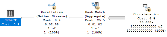
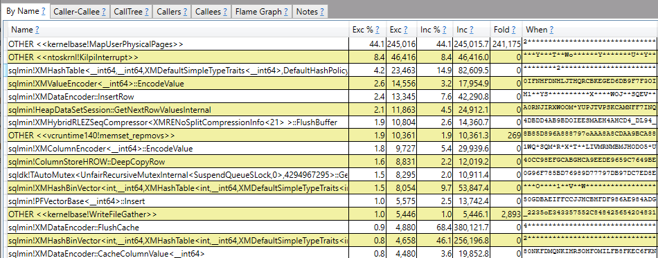
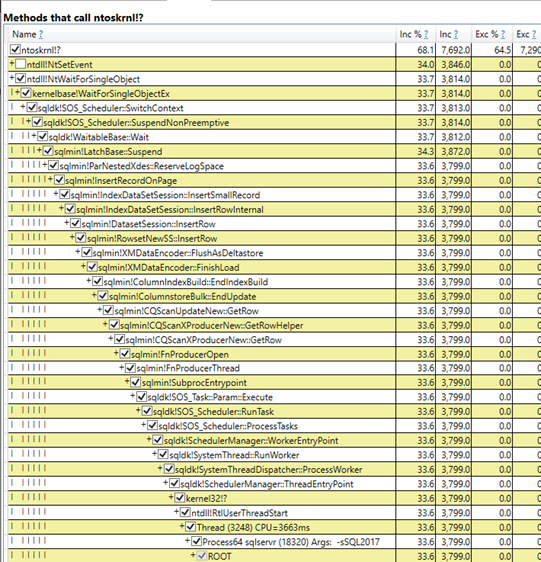
I don’t know of a more faster way to complete the challenge. Without an actual plan, the query takes about 63 seconds to complete. However, the query takes about 3 minutes to complete on SQL Server 2019, even without requesting an actual plan. The difference is caused by lightweight query profiling in SQL Server 2019, which is turned on by default. I find query profiling to be very useful in general for evaluating performance issues in real time and for estimating how long a query will take to complete. However, it can still add significant overhead for certain types of queries. The difference is quite apparent in the call stacks:
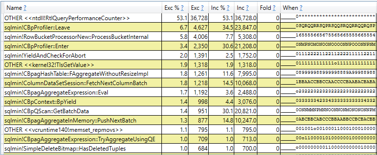
This is why I did all of my testing for this blog post on SQL Server 2017, in case you’ve been wondering that.
Final Thoughts
Summary of all attempts:
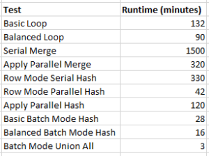
The results are quite specific to the test scenario: they should not be used to draw conclusions about general join performance. As mentioned earlier, in a few cases the bottleneck is the query profiling infrastructure instead of typical aspects of query performance. If anyone out there knows of a faster technique than those tested here, I would be delighted to learn about it.
Thanks for reading!
Going Further
If this is the kind of SQL Server stuff you love learning about, you’ll love my training. I’m offering a 75% discount to my blog readers if you click from here. I’m also available for consulting if you just don’t have time for that and need to solve performance problems quickly.