Another Method to Reduce Temp Table Plan Cache Pollution

SQL Server allows stored procedures to reference temporary tables that were created in an outer scope. However, doing so can cause the plan cache pollution problem described here.

The Polluter

The problem can be observed with a simple repro script. The child stored procedure performs a series of updates on a temp table. The parent procedure creates the temp table, calls the child stored procedure, and returns data from the temp table.

CREATE OR ALTER PROCEDURE dbo.update_temp_table
AS
BEGIN
    SET NOCOUNT ON;
    -- the #outer_scope temp table is created in an outer scope

    UPDATE #outer_scope SET CNT = (SELECT COUNT(*) FROM master..spt_values t1 CROSS JOIN master..spt_values t2) + (SELECT COUNT(*) FROM master..spt_values t1 CROSS JOIN master..spt_values t2)
    WHERE ID = 1;

    UPDATE #outer_scope SET CNT = (SELECT COUNT(*) FROM master..spt_values t1 CROSS JOIN master..spt_values t3) + (SELECT COUNT(*) FROM master..spt_values t1 CROSS JOIN master..spt_values t2)
    WHERE ID = 1;

    UPDATE #outer_scope SET CNT = (SELECT COUNT(*) FROM master..spt_values t1 CROSS JOIN master..spt_values t4) + (SELECT COUNT(*) FROM master..spt_values t1 CROSS JOIN master..spt_values t2)
    WHERE ID = 1;

    UPDATE #outer_scope SET CNT = (SELECT COUNT(*) FROM master..spt_values t1 CROSS JOIN master..spt_values t5) + (SELECT COUNT(*) FROM master..spt_values t1 CROSS JOIN master..spt_values t2)
    WHERE ID = 1;
END;

GO

CREATE OR ALTER PROCEDURE dbo.parent_proc
AS
BEGIN
    SET NOCOUNT ON;

    CREATE TABLE #outer_scope (ID INT NOT NULL, CNT INT NULL);
    INSERT INTO #outer_scope (ID, CNT)
    VALUES (1, NULL);

    EXEC dbo.update_temp_table;

    SELECT * FROM #outer_scope;
END;

GO

I executed the parent_proc procedure on three different sessions and was rewarded with three different cached plans:

The Cleaner

One way to resolve this issue is to change the child procedure to create a new local temp table, to copy the data from the original table into the new one using its own child procedure, to perform the updates against the new table, and to copy back the data into the original table, again in a child procedure. That was a lot of words so perhaps code will be easier to understand:

CREATE OR ALTER PROCEDURE dbo.update_temp_table_import_temp_data
WITH RECOMPILE
AS
BEGIN	
    IF OBJECT_ID(N'tempdb..#outer_scope', 'U') IS NOT NULL
    BEGIN
        INSERT INTO #local_scope
        SELECT * FROM #outer_scope;
    END;
END;

GO


CREATE OR ALTER PROCEDURE dbo.update_temp_table_export_temp_data
WITH RECOMPILE
AS
BEGIN
    IF OBJECT_ID(N'tempdb..#outer_scope', 'U') IS NOT NULL
    BEGIN
        TRUNCATE TABLE #outer_scope;	

        INSERT INTO #outer_scope
        SELECT * FROM #local_scope;
    END;
END;

GO


CREATE OR ALTER PROCEDURE dbo.update_temp_table_NEW
AS
BEGIN
    SET NOCOUNT ON;
    
    CREATE TABLE #local_scope (ID INT NOT NULL, CNT INT NULL);
    
    EXEC dbo.update_temp_table_import_temp_data;
    
    UPDATE #local_scope SET CNT = (SELECT COUNT(*) FROM master..spt_values t1 CROSS JOIN master..spt_values t2) + (SELECT COUNT(*) FROM master..spt_values t1 CROSS JOIN master..spt_values t2)
    WHERE ID = 1;

    UPDATE #local_scope SET CNT = (SELECT COUNT(*) FROM master..spt_values t1 CROSS JOIN master..spt_values t3) + (SELECT COUNT(*) FROM master..spt_values t1 CROSS JOIN master..spt_values t2)
    WHERE ID = 1;

    UPDATE #local_scope SET CNT = (SELECT COUNT(*) FROM master..spt_values t1 CROSS JOIN master..spt_values t4) + (SELECT COUNT(*) FROM master..spt_values t1 CROSS JOIN master..spt_values t2)
    WHERE ID = 1;

    UPDATE #local_scope SET CNT = (SELECT COUNT(*) FROM master..spt_values t1 CROSS JOIN master..spt_values t5) + (SELECT COUNT(*) FROM master..spt_values t1 CROSS JOIN master..spt_values t2)
    WHERE ID = 1;
    
    EXEC update_temp_table_export_temp_data;
END;	
    
GO


CREATE OR ALTER PROCEDURE dbo.parent_proc_NEW
AS
BEGIN
    SET NOCOUNT ON;

    CREATE TABLE #outer_scope (ID INT NOT NULL, CNT INT NULL);
    INSERT INTO #outer_scope (ID, CNT)
    VALUES (1, NULL);

    EXEC dbo.update_temp_table_NEW;

    SELECT * FROM #outer_scope;
END;

GO

Running the new procedure in three different sessions no longer results in cache pollution:

This is because the references to outer-scoped temp tables have been moved to small, simple procedures that are built with a procedure level RECOMPILE hint. This approach has the following advantages:

  • There is no cache pollution for any of the code.
  • The update statements will be compiled significantly less often, especially on SQL Server 2019 and above.

It also has the following disadvantages:

  • Data from the outer table needs to be written to the local table and data from the local table is written back to the outer table.
  • The definition and columns of the temp table need to be duplicated in additional places in code.

I don’t think that this is the best general solution by any means, but it does fulfill a particular niche use case and I’ve been able to use this method in production code. For other ideas, Erland Sommarskog has a detailed write up of different ways of passing data between procedures.

Final Thoughts

When you need your plan cache to be cleaned there’s really only one person to call:

Thanks for reading!

Improving AT TIME ZONE Performance

Queries that use the AT TIME ZONE operator may perform worse than desired. For example, Jonathan Kehayias blogged about performance struggles with AT TIME ZONE at sqlskills.com. One key difference between Jonathan’s opinion and my own is that I enjoy writing these kinds of posts.

Test Data

The test data consists of one million rows per day over the month of January 2022 for a total of 31 million rows.

DROP TABLE IF EXISTS dbo.CCIForBlog;

CREATE TABLE dbo.CCIForBlog (
    SaleTimeUTC DATETIME2 NOT NULL,
    WidgetCount BIGINT NOT NULL,
    INDEX CCI CLUSTERED COLUMNSTORE
);

GO

SET NOCOUNT ON;

DECLARE
    @StartDate DATETIME2 = '20220101',
    @DaysToLoad INT = 31,
    @DaysLoaded INT = 0;

WHILE @DaysLoaded < @DaysToLoad
BEGIN
    INSERT INTO dbo.CCIForBlog (SaleTimeUTC, WidgetCount)
    SELECT DATEADD(SECOND, q.RN / 11.5, @StartDate), q.RN / 100000
    FROM
    (
        SELECT TOP (1000000) ROW_NUMBER() OVER (ORDER BY (SELECT NULL))
        FROM master..spt_values t1
        CROSS JOIN master..spt_values t2
    ) q (RN)
    OPTION (MAXDOP 1);

    SET @StartDate = DATEADD(DAY, 1, @StartDate);
    SET @DaysLoaded = @DaysLoaded + 1;
END;

CREATE STATISTICS S1 ON CCIForBlog (SaleTimeUTC);

Data is saved to a table with a clustered columnstore index. Of course, this is a small amount of data for a columnstore table. However, it is more than sufficient to demonstrate AT TIME ZONE as a performance bottleneck.

Filtering

Suppose an end user wants a count of widgets sold between January 3rd and January 6th. A first attempt at this query could look like the following:

SELECT SUM(WidgetCount)
FROM dbo.CCIForBlog c
WHERE c.SaleTimeUTC >= '20220103'
AND c.SaleTimeUTC < '20220106'
OPTION (MAXDOP 1);

This query plays to all of columnstore’s strengths and it only takes around 10 milliseconds to execute. The data was loaded in date order so most of the rowgroups are eliminated. However, end users don’t think in terms of UTC time. The end user actually wanted Central Standard Time. After a bit of research, the query is changed to as follows:

SELECT SUM(WidgetCount)
FROM dbo.CCIForBlog c
WHERE SWITCHOFFSET(c.SaleTimeUTC, 0) AT TIME ZONE 'Central Standard Time' >= '20220103'
AND SWITCHOFFSET(c.SaleTimeUTC, 0) AT TIME ZONE 'Central Standard Time' < '20220106'
OPTION (MAXDOP 1);

The AT TIME ZONE operator is useful when the number of offset minutes is unknown. UTC always has an offset of 0 so it is better to use SWITCHOFFSET(datetimeoffset_expression, 0)as opposed to AT TIME ZONE ‘UTC’. Even so, the query still takes over 3 minutes to execute on my machine. Nearly all of the execution time is spent on performing AT TIME ZONE calculations:

Note that using c.SaleTimeUTC AT TIME ZONE 'UTC' AT TIME ZONE 'Central Standard Time' would double the execution time.

One idea is to rewrite the filtering so that the time zone conversions are done on the constant values instead of the column:

WHERE c.SaleTimeUTC >= SWITCHOFFSET('20220103' AT TIME ZONE 'Central Standard Time', 0)
AND c.SaleTimeUTC < SWITCHOFFSET('20220106' AT TIME ZONE 'Central Standard Time', 0)

I strongly recommend against this approach. It can lead to wrong results for some time zones and boundary points. Instead, you can use the fact that datetimeoffset only supports an offset of up to +-14 hours. That means that (local – 14 hours) < UTC < (local + 14 hours) is true for any time zone and any point in time. A logically redundant filter can be added to the query:

SELECT SUM(WidgetCount)
FROM dbo.CCIForBlog c
WHERE SWITCHOFFSET(c.SaleTimeUTC, 0) AT TIME ZONE 'Central Standard Time' >= '20220103'
AND SWITCHOFFSET(c.SaleTimeUTC, 0) AT TIME ZONE 'Central Standard Time' < '20220106'
AND c.SaleTimeUTC >= DATEADD(HOUR, -14, '20220103')
AND c.SaleTimeUTC < DATEADD(HOUR, 14, '20220106')
OPTION (MAXDOP 1);

The newly improved query finishes in around 26 seconds. It is able to benefit from rowgroup elimination and performs significantly fewer time zone conversions compared to the original query. In this case, we were able to use knowledge about time zones and a bit of date math to improve performance from over 3 minutes to about 26 seconds.

Grouping

Suppose that an end user wants widget counts summarized by date. A first attempt at this query could look like the following:

SELECT ca.ConvertedDate, SUM(WidgetCount)
FROM dbo.CCIForBlog c
CROSS APPLY (
    SELECT CAST(c.SaleTimeUTC AS DATE)
) ca (ConvertedDate)
GROUP BY ca.ConvertedDate
OPTION (MAXDOP 1);

This query takes about 1 second on my machine. However, once again, the end user wants the data to be in CST instead of UTC. The following approach takes around 3 minutes:

SELECT ca.ConvertedDate, SUM(WidgetCount)
FROM dbo.CCIForBlog c
CROSS APPLY (
    SELECT CAST(SWITCHOFFSET(c.SaleTimeUTC, 0) AT TIME ZONE 'Central Standard Time' AS DATE)
) ca (ConvertedDate)
GROUP BY ca.ConvertedDate
OPTION (MAXDOP 1);

This should not be a surprise because the bottleneck in query performance is performing 31 million AT TIME ZONE calculations. That doesn’t change if the query performs filtering or grouping.

Historically, governments only perform daylight saving time or offset switches on the minute. For example, an offset won’t change at 2:00:01 AM, but it might change at 2:00:00 AM. The source data has one million rows per day, so grouping the date truncated to the minute, applying the time zone conversion to the truncated distinct values, and finally grouping by date should lead to significant performance improvement. One way to accomplish this:

SELECT ca.ConvertedDate, SUM(SumWidgetCount)
FROM 
(
    SELECT DATEADD(MINUTE, DATEDIFF(MINUTE, '20000101', c.SaleTimeUTC), '20000101'), SUM(WidgetCount)
    FROM dbo.CCIForBlog c
    GROUP BY DATEADD(MINUTE, DATEDIFF(MINUTE, '20000101', c.SaleTimeUTC), '20000101')
) q (SaleTimeUTCTrunc, SumWidgetCount)
CROSS APPLY (
    SELECT CAST(SWITCHOFFSET(q.SaleTimeUTCTrunc, 0) AT TIME ZONE 'Central Standard Time' AS DATE)
) ca (ConvertedDate)
GROUP BY ca.ConvertedDate
OPTION (MAXDOP 1);

The new query takes around 4 seconds on my machine. It needs to perform 44650 time zone conversions instead of 31 million. Once again, we were able to use knowledge about time zones and a bit of date math to improve performance.

Functioning

I’ve developed and open sourced replacement functions for AT TIME ZONE to provide an easier way of improving performance for queries that use AT TIME ZONE. The TZGetOffsetsDT2 function returns a pair of offsets and the TZFormatDT2 function transforms those offsets into the desired data type. The filtering query can be written as the following:

SELECT SUM(WidgetCount)
FROM dbo.CCIForBlog c
OUTER APPLY dbo.TZGetOffsetsDT2 (c.SaleTimeUTC, N'UTC', N'Central Standard Time') o
CROSS APPLY dbo.TZFormatDT2 (c.SaleTimeUTC, N'UTC', N'Central Standard Time', o.OffsetMinutes, o.TargetOffsetMinutes) f
WHERE f.ConvertedDateTime2 >= '20220103'
AND f.ConvertedDateTime2 < '20220106'
OPTION (MAXDOP 1);

The new query takes around 10 seconds to execute. The new query plan is able to use batch mode processing at every step:


If desired, performance can be further improved by adding the same redundant filters as before:

SELECT SUM(WidgetCount)
FROM dbo.CCIForBlog c
OUTER APPLY dbo.TZGetOffsetsDT2 (c.SaleTimeUTC, N'UTC', N'Central Standard Time') o
CROSS APPLY dbo.TZFormatDT2 (c.SaleTimeUTC, N'UTC', N'Central Standard Time', o.OffsetMinutes, o.TargetOffsetMinutes) f
WHERE f.ConvertedDateTime2 >= '20220103'
AND f.ConvertedDateTime2 < '20220106'
AND c.SaleTimeUTC >= DATEADD(HOUR, -14, '20220103')
AND c.SaleTimeUTC < DATEADD(HOUR, 14, '20220106')
OPTION (MAXDOP 1);

The most optimized version takes around 1 second to execute. Quite an improvement compared to 3 minutes!

The grouping query can also be rewritten using the new functions:

SELECT f.ConvertedDate, SUM(WidgetCount)
FROM dbo.CCIForBlog c
OUTER APPLY dbo.TZGetOffsetsDT2 (c.SaleTimeUTC, N'UTC', N'Central Standard Time') o
CROSS APPLY dbo.TZFormatDT2 (c.SaleTimeUTC, N'UTC', N'Central Standard Time', o.OffsetMinutes, o.TargetOffsetMinutes) f
GROUP BY f.ConvertedDate
OPTION (MAXDOP 1);

This version takes about 7 seconds to execute. This is slower than the date truncation method which took 4 seconds but still much faster than the original AT TIME ZONE method.

Unfortunately, SQL Server limitations require a pair of functions to get the best performance. The open source project does provide a simpler function that can be called by itself but it is only eligible for nested loop joins.

Upgrading

SQL Server 2022 RC1 has signs of improvement for AT TIME ZONE. The basic queries that use AT TIME ZONE in this blog post take about 75 seconds to execute on my machine, so it could be estimated that SQL Server 2022 will reduce the CPU footprint of AT TIME ZONE by 60%. Release candidates are not fully optimized so it’s possible that final performance numbers will be different once the product goes GA. I suspect that these performance improvements are already present in Azure SQL Database but I can’t find any documentation for the change.

Final Thoughts

Please try my open source project if you’re experiencing performance problems with AT TIME ZONE. Thanks for reading!

Why Parallel Queries are Sometimes Slow In SQL Server

You may have noticed large variations in elapsed time for parallel queries while performing query tuning or observing a production workload. This post reviews some of the possible explanations for those variations. I’m testing on SQL Server 2022 RC0 but this behavior can be observed on all currently supported versions of SQL Server.

The Setup

The test data is very simple. Insert ten million sequential integers into a single column table with a clustered index:

CREATE TABLE dbo.ParallelTest (
Id BIGINT NOT NULL,
CONSTRAINT PK_ParallelTest PRIMARY KEY (Id)
);

INSERT INTO dbo.ParallelTest (Id)
SELECT [value]
FROM GENERATE_SERIES(1, 10000000);

Now consider the following query:

SELECT SUM(a.ID + b.ID) s
FROM dbo.ParallelTest a
INNER JOIN dbo.ParallelTest b ON a.ID = b.ID
OPTION (USE HINT ('DISALLOW_BATCH_MODE'));

The query optimizer naturally picks a merge join for this query. The self-joined tables obviously have the same row count and the data is already sorted. That makes this query an ideal candidate for a serial merge join from the optimizer’s point of view . The USE HINT in the query isn’t particularly important and the example works without it, but its presence will be explained later. Here’s what the query plan looks like for me:

The query takes 2721 ms of CPU time and elapsed time to execute on my machine. It’s reasonable for CPU and elapsed time to match here because there’s nothing for the query to wait on. It’s the only user query running against the SQL instance. Next I’ll force a parallel merge join query plan by changing the query hints to the following:

SELECT SUM(a.ID + b.ID) s
FROM dbo.ParallelTest a
INNER JOIN dbo.ParallelTest b ON a.ID = b.ID
OPTION (MAXDOP 8, MERGE JOIN, USE HINT('ENABLE_PARALLEL_PLAN_PREFERENCE', 'DISALLOW_BATCH_MODE'));

I chose MAXDOP 8 because my test machine has 8 physical CPU cores. This is an unnatural query plan with a higher parallel cost than serial cost. The query optimizer only picked it because it was forced to. Note the presence of the exchange operators with a relatively high estimated cost:

The parallel query takes 6465 ms of CPU time and 1723 ms of elapsed time to execute on my machine. It finished about 33% faster than the serial query but CPU time more than doubled. The exchange operators added a large overhead for this query. Next I’ll run the same query again but I’ll make one of my CPUs busier than before. Consider the following infinite loop coded as a stored procedure:

CREATE OR ALTER PROCEDURE #p AS
SET NOCOUNT ON;
DECLARE @i INT;
WHILE 1 = 1
SET @i = 0;
GO

EXEC #p;

This code does not accomplish anything besides efficiently using CPU resources, which is exactly what I need for my test. I’m running the merge query at MAXDOP 8 on a machine with 8 CPU cores so I’m pretty much guaranteed to see scheduler contention for some of the workers of the parallel query. They will compete for CPU resources with the infinite loop.

Take a moment to predict the performance penalty that the parallel query will experience due to the busy scheduler. Will it be 2X slower? 3X slower? Worse? For a few hints, recall that hash distributed exchange operators will generally try to force an equal amount of work to each thread. Also recall that a parallel merge join requires order-preserving exchange operators. I’ve included Erik running at MAXDOP 8 to hopefully prevent you from accidentally seeing the answer before you’ve finalized your prediction.

With the busy scheduler, the query now takes 6818 ms of CPU time and 31745 ms of elapsed time to execute on my machine. The same code is over 18X slower simply due to the highly efficient stored procedure that’s running on the same SQL instance. Here are the query wait stats in case they are of interest:

<Wait WaitType=”CXPACKET” WaitTimeMs=”454673″ WaitCount=”5262″ />
<Wait WaitType=”CXSYNC_PORT” WaitTimeMs=”32539″ WaitCount=”41″ />
<Wait WaitType=”CXSYNC_CONSUMER” WaitTimeMs=”43″ WaitCount=”14″ />

scheduler_ring_buffer_recorded

This is an inappropriately brief introduction to a complex topic, but workers cooperate with each other by sharing time on schedulers. Under normal conditions, a worker will execute code on the scheduler for up to 4 milliseconds before yielding. The worker yields in case there’s another worker waiting to execute on the scheduler. When there’s not the original worker immediately starts executing code again. An example of when a worker yields early is if it needs to wait for an I/O operation.

scheduler_ring_buffer_recorded is the name of a debug extended event that you should probably never use. I often don’t follow my own advice, so I used it to get an idea of how often workers were yielding to the scheduler for the merge join queries. I only looked at action types of “SCHEDULER_NONPREEMPTIVE_RESUME” and I admit that this analysis is quite approximate. For the MAXDOP 1 query, there was a total of 705 events over 2872 milliseconds. In other words, the average time spent on the scheduler before yielding is close to the 4 ms soft maximum. This should be expected for the serial query if all of the data is in the buffer pool. There is no memory grant for the query (the reason for the USE HINT) and there’s not really any reason to yield early.

The parallel query had significantly more yields. Looking at one worker thread as an example, it had 14862 events over 1714 milliseconds. In other words, it had around 35 times the number of scheduler yields compared to the MAXDOP 1 query. The higher number of yields is a performance liability when competing with workers from other queries on the same scheduler. The infinite loop stored procedure dominates the workers from the parallel and gets around 97% of the cpu time on the scheduler. That’s a big part of why the parallel query is 18X slower than before.

Note that you can also get this information by looking at the yield_count column of the sys.dm_of_schedulers DMV, but those numbers are server wide and aren’t isolated to one query. With that said, I did get reasonably similar results when comparing that column to the extended event results.

To summarize, parallel query performance overhead isn’t as simple as just the direct overhead of the exchange operators. A query changing from serial to parallel can result in completely different interactions between the workers and the scheduler. The serial query executed its code 4 milliseconds at a time. The parallel query had to yield significantly more often. This type of change isn’t something that you can directly observe in a query plan.

Why Parallel Queries are Sometimes Slow

There are many reasons why a parallel query may not be as efficient as you hoped. I find these to be the most common:

1) There is an overhead associated with parallel exchange operators which is not present in serial queries. Moving data between worker threads requires additional CPU time which adds to the overall execution time of the query. I believe this is what is described by the following quote from the documentation:

Simple queries, frequently found in transaction processing applications, find the additional coordination required to execute a query in parallel outweigh the potential performance boost.

2) There’s some kind of additional coordination required between threads which delays query completion. For example, an order-preserving repartition streams operator is generally worse for performance than one that doesn’t need to preserve order. A different type of example can be seen in my blog post about slow parallel scans caused by cloud storage.

3) Work may be unevenly distributed between worker threads. For example, an eager index spool can only be built with one thread. Other threads may be idle while that temporary index is built. For a different example, a filtered parallel scan of a table may not output the same number of rows to all threads. All else being equal, a parallel query that cannot use all of the CPUs allowed by MAXDOP is not as efficient as one that can.

4) Work may be evenly distributed between worker threads but some of the CPUs are busier than others. Some parallel queries are as slow as their busiest CPU, even when queries are evenly sharing time on the scheduler. Of course, dramatic performance penalties can be seen when the parallel query gets an uneven amount of time on the scheduler (like in the demo in this blog post).

Mitigations

Individual parallel query performance can degrade due to contention on a single scheduler that’s used by one or more of its workers. You are more likely to run into problems with higher DOP or a higher number of concurrent queries. Lowering MAXDOP decreases the odds that you’ll run into the worst type of contention because the query uses fewer schedulers. Decreasing the number of queries decreases contention per scheduler which also helps.

To explain it in a different way, the simplest way to reduce problems with parallel queries is to have fewer worker threads per scheduler. This is of course a balancing act, but it’s one that you must perform for some workloads. Set Cost Threshold for Parallelism and server/database/resource governor MAXDOP appropriately. When possible, don’t run too many concurrent queries for your hardware.

For very important queries for which performance is critical, consider changing to a type of parallelism that isn’t as susceptible to scheduler contention issues. The two most common methods are a parallel apply pattern, perhaps using demand partitioning, or batch mode execution.

Batch mode is yet another complicated topic that I’m not going to explain here, but it uses a fundamentally different method of parallelism compared to row-mode execution which is generally much more robust against problems caused by busy schedulers. Below is a comparison of elapsed times with and without the infinite loop stored procedure running:

The elapsed time of the parallel batch mode query only changes slightly. This is also a nice property when considering overall server scalability.

Final Thoughts

I was going to originally blog about DOP feedback, but it’s taking a while for my feedback to kick in. Thanks for reading!

Ordered Columnstore Indexes on SQL Server 2022 CTP 2.0

Brent recently blogged about ordered columnstore indexes in SQL Server 2022 and had some trouble with them, so I decided to take a look into the mechanics of the feature. I’m testing on SQL Server 2022 CTP 2.0.

What does the ordered columnstore feature do?

  1. A sort operator may be added to query plans that insert into the table. The sort operator is a bit unusual in that the data may not be fully sorted.
  2. A sort operator is added when initially creating an ordered columnstore index. The level of rowgroup elimination fragmentation will depend on memory, DOP, and other factors.
  3. A sort operator is added when rebuilding an ordered columnstore index. The level of rowgroup elimination fragmentation will depend on memory, DOP, and other factors.

Technical details for insert

The sort for inserting into an ordered columnstore is a DML request sort. It appears to use the same internal mechanism as the sort that’s added for inserting into partitioned columnstore tables. The difference is that the data is sorted by the specified columns instead of a calculated partition id. In my testing, the sort appears to be a best effort sort that does not spill to tempdb. This means that if SQL Server thinks there won’t be enough memory then the data will not be fully sorted. Parallel inserts have an additional complication. Consider the following query plan image:

That is a row mode sort. It is a row mode sort because a batch mode parallel sort would put all resulting rows on a single thread which would make the parallel insert pointless. However, there’s no repartition streams operator as a child of the sort. Data is sorted on each thread in a best effort fashion. Even if there is enough memory to fully sort the data, you will end up with DOP threads of sorted data instead. The data will not be sorted globally. The split into threads will increase rowgroup elimination fragmentation.

As mentioned earlier, the sort operator does not always appear. It is not present when the cardinality estimate is very low (around 250 rows). I suspect that the same logic is used for adding the sort as adding the memory grant for compression. For very low cardinality estimates, the data will be inserted into delta rowgroups, even if there’s more than 102399 rows. By that same reasoning, I expect that there is no sort operator if the INSERT query hits a memory grant timeout.

For more information on this sort, see CQScanPartitionSortNew in Paul White’s blog post about different sort types in SQL Server.

Technical details for CREATE/REBUILD index

I spent less time looking into the sort that’s added as part of CREATE or REBUILD index. In my testing, the sort again does not spill to tempdb. The sort is also performed on a per thread basis for parallel index operations. The minimum fragmentation level will be achieved for a MAXDOP 1 operation with sufficient memory. Reducing memory or running the create index in parallel will increase fragmentation. This is unfortunate because ordered columnstore indexes do not support online index creation or rebuilds.

An unpopular opinion

I think that the community worries too much with columnstore with respect to achieving perfect segment ordering and keeping rowgroups at exactly 1048576 rows. If you perform basic maintenance and partition tables appropriately then that should be good enough for most data warehouse workloads. Most query performance issues are going to be caused by getting no elimination at all, scanning through too many soft-deleted rows, or the usual query performance problems. Scanning 11 rowgroups instead of 5 probably isn’t why your queries on columnstore indexes are slow today.

Final thoughts

As is, this feature can be described as a poor man’s partitioning. The sweet spot for this functionality feels very limited to me in its current state, but we’re still on CTP 2.0. Maybe there will be changes before RTM. Thanks for reading!

TRY_CAST and TRY_PARSE Can Return Different Results

There’s a lot of guidance out there that states that TRY_CAST is a faster, more modern version of TRY_PARSE and that TRY_PARSE should only be used if you need to set the optional culture parameter. However, the two functions can return different results in some cases, even without the culture parameter.

Parsing

First I’ll throw a million rows into a single varchar column temp table:

CREATE TABLE #number_as_string (why_tho VARCHAR(100));

INSERT INTO #number_as_string (why_tho)
SELECT ISNULL(CAST(TRY_CAST(q.RN % 33000 AS SMALLINT) AS VARCHAR(100)), '')
FROM
(
	SELECT TOP (1000000) ROW_NUMBER() OVER (ORDER BY (SELECT NULL)) RN
	FROM master..spt_values t1
	CROSS JOIN master..spt_values t2
) q;

Let’s suppose that I want to count the rows that are numbers that fit within the limits of the TINYINT data type. The following code takes 36937 ms of CPU time on my machine and returns a value of 7935:

SELECT COUNT_BIG(*)
FROM #number_as_string
WHERE TRY_PARSE(why_tho AS TINYINT) IS NOT NULL
OPTION (MAXDOP 1);

The poor performance of the query isn’t unexpected. The documentation mentions the following about TRY_PARSE:

Keep in mind that there is a certain performance overhead in parsing the string value.

Casting

I can use TRY_CAST in an attempt to avoid the string parsing overhead of TRY_PARSE. The following code uses 110 ms of CPU time so it is significantly faster than the previous query:

SELECT COUNT_BIG(*)
FROM #number_as_string
WHERE TRY_CAST(why_tho AS TINYINT) IS NOT NULL
OPTION (MAXDOP 1);

However, this query returns a value of 14895, nearly double the count from before. The query results are different because TRY_PARSE returns NULL for an empty string but TRY_CAST returns 0. As a workaround (special thanks to Stephen Morris), the following query returns the expected value of 7935 and completes after using 157 ms of CPU time:

SELECT COUNT_BIG(*)
FROM #number_as_string
WHERE TRY_CAST(why_tho AS TINYINT) IS NOT NULL AND why_tho NOT IN ('', '+', '-')
OPTION (MAXDOP 1);

Final Thoughts

It’s not that TRY_CAST is returning the wrong results. In SQL Server, an empty string converts to 0 when cast to an integer data type. It’s more so that when TRY_CAST is applied to a string, the person writing the query usually wants only the values that a human would consider to be a number. TRY_PARSE seems to follow a set of rules that is more in line with human judgment of what is and isn’t a number. Avoiding TRY_PARSE due to the performance penalty is still a good idea in many cases, but be sure to filter out empty strings if you don’t want them included in the result set. If anyone knows of any other values treated differently between TRY_CAST and TRY_PARSE kindly leave a comment on this blog post. Thanks for reading!

Unkillable Sessions and Undetected Deadlocks

I recently experienced a blocking issue in a production environment which had been going on for hours. As a responsible DBA, I tried to kill the head of the blocking chain. Unexpectedly, killing the session seemed to have no effect. The blocking continued and the session seemed to stick around.

How to Create an Unkillable Session

It’s surprisingly easy to create a session that seemingly can’t be killed. Use good judgment in picking an environment to run this code against. First you’ll need to enable the “Ad Hoc Distributed Queries” configuration option if you haven’t done so already:

sp_configure 'Ad Hoc Distributed Queries', 1;
RECONFIGURE;
GO
sp_configure;

You can then run the following code after replacing the SERVER_NAME and INSTANCE_NAME placeholder values with the server name and instance name that you’re running against. In other words, you want the OPENROWSET call to point at the same server that you’re executing the query against:

BEGIN TRANSACTION;

SELECT TOP (1) [name]
FROM master.dbo.spt_values WITH (TABLOCKX);

SELECT TOP (1) d.[name]
FROM OPENROWSET('SQLNCLI', '{{SERVER_NAME}}\{{INSTANCE_NAME}};Trusted_Connection=yes;', master.dbo.spt_values) AS d;

This code seems to run forever. Trying to kill the session is not effective, even though there’s no error message and a line written to the error log claiming that the session was killed. Running kill with the STATUSONLY option gives us the following:

SPID 56: transaction rollback in progress. Estimated rollback completion: 0%. Estimated time remaining: 0 seconds.

Trying to cancel the query using SSMS also seems to have no effect as well.

The Undetected Deadlock

Running sp_whoisactive reveals a pretty alarming state:

Session 56 (the one that I can see in SSMS) is waiting on an OLEDB wait. Based on the documentation, I assume that you’ll get this wait type while waiting for the OPENROWSET call to complete:

Includes all connection information that is required to access remote data from an OLE DB data source. This method is an alternative to accessing tables in a linked server and is a one-time, ad hoc method of connecting and accessing remote data by using OLE DB.

I did get callstacks for the OLEDB wait using the wait_info_external extended event, but there were two problems. The first problem is that wait_info_external fires after the wait is complete and the OLEDB wait won’t finish. The second problem is that the callstacks that I did get weren’t very interesting.

Getting back on topic, I believe that the OLEDB wait for session 56 can only end once session 66 completes its work. Session 66 is the session that was created by the OPENROWSET call. However, session 66 needs an IS lock on the spt_values table. That is not compatible with the exclusive lock held on that object by session 56. So session 56 is waiting on session 66 but session 66 is waiting on session 56. This is an undetected deadlock. The deadlock can be resolved by killing session 66 (the OPENROWSET query).

Note that if you are crazy enough to try this on your own, you may see a MEMORY_ALLOCATION_EXT wait instead of an OLEDB wait. I don’t believe that there’s any meaningful distinction there, but don’t assume that a long running OLEDB wait is required for this problem to occur.

Final Thoughts

This blocking issue was unusual in that killing the blocking session doesn’t resolve the issue. I had to kill the session getting blocked instead. Thanks for reading!

Why Some Types of Parallel Scans can be Slow on Cloud Storage

Upon reading the title, you may be thinking that of course parallel scans will be slow in the cloud. Cloud storage storage simply isn’t very fast. I would argue that there’s a bit more to it.

The Timeout

A query timed out the other day in production after running for 600 seconds. Of note, one of the tables used by the stored procedure is in a database with data files hosted by Azure blob storage. I grabbed the wait stats for the timed out query using query store:

According to the documentation, the latch category maps to LATCH_% wait types and the preemptive category maps to PREEMPTIVE_% wait types. I wasn’t able to reproduce the timeout when executing the same query text, even if I forced the exact same query plan with a USE PLAN. Admittedly, I was puzzled by the wait stats distribution for a while.

Decoding the Categories

I eventually realized that typically the first execution of the stored procedure for the business day tended to be the slowest. Sorting query store runtime DMV results by time:

I also noticed that the timed out executions tended to have higher physical I/O than the other executions. Sorting query store runtime DMV results by I/O:

I now finally had a method to reproduce the poor performance of the stored procedure: being the first one to run the code in the morning, presumably when the buffer pool didn’t have anything helpful for this stored procedure. Early in the morning, I was able to capture an actual plan that took 13 minutes at MAXDOP 8. Nearly all of the execution time is spent on an index scan for a table that is hosted on cloud storage:

Here are the top wait stats from the actual plan:

<Wait WaitType=”LATCH_EX” WaitTimeMs=”5423928″ WaitCount=”1971″ />
<Wait WaitType=”PAGEIOLATCH_SH” WaitTimeMs=”977288″ WaitCount=”29210″ />
<Wait WaitType=”CXPACKET” WaitTimeMs=”809678″ WaitCount=”700″ />
<Wait WaitType=”PREEMPTIVE_HTTP_REQUEST” WaitTimeMs=”43801″ WaitCount=”50344″ />

I used the task DMVs during query execution to get information about the latch type:


Now I know that the query spends most of its time trying to acquire exclusive latches of the ACCESS_METHODS_DATASET_PARENT type. There is also a fair amount of I/O wait time compared to the mysterious PREEMPTIVE_HTTP_REQUEST wait type.

The ACCESS_METHODS_DATASET_PARENT Latch

I asked the community if this latch was considered to be interesting. The winning option was “What?”. As usual, twitter is useless:

For my query, at times I observed seven out of eight worker threads all waiting for an exclusive latch at the same time. This isn’t surprising considering that the query averaged 6.7 LATCH_EX wait seconds per second. That the other thread was doing an I/O wait while the others were waiting for the latch, so perhaps the worker threads were doing I/Os while holding the latch resource. On a development environment (with unfortunately significantly better I/O), I mocked up a roughly similar table and enabled the latch_acquired, latch_released, file_read, and file_read_completed extended events. The results were quite educational:

There were two different patterns in the XE files. Sometimes the worker threads would acquire the latch, perform one or more I/Os, and release the latch. Otherwise they would acquire the latch and quickly release it without performing any I/Os. Paul Randal recently wrote the following about this latch:

When either a heap or an index is being accessed, internally there’s an object called a HeapDataSetSession or IndexDataSetSession, respectively. When a parallel scan is being performed, the threads doing the actual work of the scan each have a “child” dataset (another instance of the two objects I just described), and the main dataset, which is really controlling the scan, is called the “parent.”

When one of the scan worker threads has exhausted the set of rows it’s supposed to scan, it needs to get a new range by accessing the parent dataset, which means acquiring the ACCESS_METHODS_DATASET_PARENT latch in exclusive mode. While this can seem like a bottleneck, it’s not really, and there’s nothing you can do to stop the threads performing a parallel scan from occasionally showing a LATCH_EX wait for this latch.

At a very high level, I suspect that the fast latch releases (marked in blue in the above picture) occur when the worker thread can acquire an already available range of rows from the parent object. The slow latch releases (marked in red) occur when the worker thread tries to acquire a new range, can’t find one, and has to perform I/Os to add more ranges to the parent object. In both cases the parent object needs to be modified, so an exclusive latch is always taken. I don’t know how it actually works behind the scenes, but the theory matches the observed behavior.

In summary, the query does a parallel scan which is protected by the ACCESS_METHODS_DATASET_PARENT latch. The table getting scanned is hosted on cloud storage with high I/O latency. Latency being high contributes to the exclusive latch on ACCESS_METHODS_DATASET_PARENT getting held for a long time which can block all of the other parallel worker threads from proceeding.

The PREEMPTIVE_HTTP_REQUEST Wait Type

I already have enough information to be confident in a query tuning fix for the stored procedure, but for completeness, I also investigated the PREEMPTIVE_HTTP_REQUEST wait type. I was not able to find any useful documentation for this wait type. The official documentation only says “Internal use only.” Thanks, Microsoft.

A common technique to learn more about undocumented waits is to get callstacks associated with the wait type. I’ve seen the PREEMPTIVE_HTTP_REQUEST wait occur in Azure SQL databases, Azure SQL Managed Instances, and for databases hosted in Azure blob storage. It is possible to get callstacks for managed instances, but it is not possible to translate them because Microsoft does not release public symbols for managed instances. However, the blob storage scenario did allow me to get and translate call stacks for the wait. Below are a few of the stacks that I captured:

Performing I/Os to read data not in the buffer pool:

sqldk!XeSosPkg::wait_info_external::Publish
sqldk!SOS_Task::PushWait
sqlmin!SOS_Task::AutoSwitchPreemptive::AutoSwitchPreemptive
sqlmin!BlobAccess::AsyncHttpIOInternal
sqlmin!BlobAccess::AsyncIOInternal
sqlmin!XFCB2::ScatterReadInternal
sqlmin!FCB::ScatterRead
sqlmin!RecoveryUnit::ScatterRead
sqlmin!BPool::GetFromDisk
sqlmin!BPool::Get
sqlmin!BlobBase::FixNode
sqlmin!BlobManager::LocateBlob
sqlmin!BlobManager::OpenInternal
sqlmin!BlobManager::Open
sqlmin!LockBytesSS::Open
sqlmin!OpenLockBytesNew
sqlmin!OpenIlbssWithSeLobHandleRO
sqlmin!IndexDataSetSession::OpenStreamWithSeLobHandle
sqlmin!RowsetNewSS::OpenWithSeLobHandle
sqlmin!CBlobHandleBaseTableFactory::PilbGet
sqlTsEs!CompareLegacyLobNull
sqlTsEs!CTEsCompare<35,35>::BlCompareXcArgArgImpl
sqlTsEs!CEsExec::GeneralEval4
sqlmin!CQScanStreamAggregateNew::GetRowHelper

Writing LOB data to disk:

sqldk!XeSosPkg::wait_info_external::Publish
sqldk!SOS_Task::PushWait
sqlmin!SOS_Task::AutoSwitchPreemptive::AutoSwitchPreemptive
sqlmin!BlobAccess::AsyncHttpIOInternal
sqlmin!BlobAccess::AsyncIOInternal
sqlmin!XFCB2::ScatterReadInternal
sqlmin!FCB::ScatterRead
sqlmin!RecoveryUnit::ScatterRead
sqlmin!BPool::GetFromDisk
sqlmin!BPool::Get
sqlmin!BlobBase::FixNode
sqlmin!Blob::RWBlob
sqlmin!Blob::RWBlob
sqlmin!Blob::ReadWriteAt
sqlmin!BlobManager::ReadAtInternal
sqlmin!BlobManager::ReadAt
sqlmin!LockBytesSS::ReadAt
sqllang!write_LOB_chunked
sqllang!`anonymous namespace’::TSendRowClassNoCount<7,0>::TSendUnlimitedVartype<0>
sqllang!CTds74::SendRowImpl
sqlTsEs!CEsExec::GeneralEval
sqllang!CXStmtQuery::ErsqExecuteQuery
sqllang!CXStmtSelect::XretExecute
sqllang!CMsqlExecContext::ExecuteStmts<1,1>

Transaction log writes:

sqldk!XeSosPkg::wait_info_external::Publish
sqldk!SOS_Scheduler::UpdateWaitTimeStats
sqldk!SOS_Task::PopWait
sqlmin!SOS_ExternalAutoWait::~SOS_ExternalAutoWait
sqlmin!SOS_Task::AutoSwitchPreemptive::~AutoSwitchPreemptive
sqlmin!BlobAccess::AsyncHttpIOInternal
sqlmin!BlobAccess::AsyncIOInternal
sqlmin!XFCB2::AsyncWriteInternal
sqlmin!FCB::AsyncWrite
sqlmin!SQLServerLogMgr::FlushLCOld
sqlmin!SQLServerLogMgr::LogWriter
sqldk!SOS_Task::Param::Execute
sqldk!SOS_Scheduler::RunTask
sqldk!SOS_Scheduler::ProcessTasks
sqldk!SchedulerManager::WorkerEntryPoint
sqldk!SystemThreadDispatcher::ProcessWorker
sqldk!SchedulerManager::ThreadEntryPoint
KERNEL32.DLL+0x0000000000017974
ntdll.dll+0x000000000006A271

I’m guessing this one is renewing the lease as noted in the documentation: “the implementation of SQL Server Data Files in Azure Storage feature requires a renewal of blob lease every 45 to 60 seconds implicitly”

sqldk!XeSosPkg::wait_info_external::Publish
sqldk!SOS_Task::PushWait
sqlmin!SOS_Task::AutoSwitchPreemptive::AutoSwitchPreemptive
sqlmin!BlobAccess::AsyncHttpIOInternal
sqlmin!BlobAccess::AsyncIOInternal
sqlmin!LeaseRenewalManager2::RenewLeases
sqlmin!XStoreLeaseRenewalTask2
sqldk!SOS_Task::Param::Execute
sqldk!SOS_Scheduler::RunTask
sqldk!SOS_Scheduler::ProcessTasks
sqldk!SchedulerManager::WorkerEntryPoint
sqldk!SystemThreadDispatcher::ProcessWorker
sqldk!SchedulerManager::ThreadEntryPoint

Not surprisingly, all of them have to do with accessing azure storage. I was able to observe an interesting pattern during a table scan: every PAGEIOLATCH_SH wait was immediately preceded by a PREEMPTIVE_HTTP_REQUEST wait.

Getting stacks for the waits that are close together, with shared code removed and the I/O wait on top with the preemptive wait on the bottom:

sqldk!XeSosPkg::wait_info::Publish
sqldk!SOS_Task::PreWait
sqldk!WaitableBase::Wait
sqlmin!LatchBase::Suspend
sqlmin!LatchBase::AcquireInternal
sqlmin!BUF::AcquireLatch
sqlmin!BPool::Get
<<SHARED STACKS REMOVED>>

sqldk!XeSosPkg::wait_info_external::Publish
sqldk!SOS_Task::PushWait
sqlmin!SOS_Task::AutoSwitchPreemptive::AutoSwitchPreemptive
sqlmin!BlobAccess::AsyncHttpIOInternal
sqlmin!BlobAccess::AsyncIOInternal
sqlmin!XFCB2::ScatterReadInternal
sqlmin!FCB::ScatterRead
sqlmin!RecoveryUnit::ScatterRead
sqlmin!BPool::GetFromDisk
sqlmin!BPool::Get
sqlmin!BlobBase::FixNode
sqlmin!BlobManager::LocateBlob
sqlmin!BlobManager::OpenInternal
sqlmin!BlobManager::Open
sqlmin!LockBytesSS::Open
sqlmin!OpenLockBytesNew
sqlmin!OpenIlbssWithSeLobHandleRO
sqlmin!IndexDataSetSession::OpenStreamWithSeLobHandle
sqlmin!RowsetNewSS::OpenWithSeLobHandle
sqlmin!CBlobHandleBaseTableFactory::PilbGet
sqlTsEs!CompareLegacyLobNull

My understanding is that SQL Server makes an HTTP request to the blob storage in preemptive mode in order to queue an asynchronous I/O. The preemptive wait ends and the PAGEIOLATCH_SH wait begins shortly after. The traditional I/O wait ends when the I/O is received by SQL Server. That’s just a guess though.

I think a reasonable summary is that you should expect to see PREEMPTIVE_HTTP_REQUEST waits if you’re performing I/O against Azure storage. They are a normal part of SQL Server’s operations.

Reducing ACCESS_METHODS_DATASET_PARENT Latch Wait Time

In some situations, a query that is slow due to I/O performance can run faster with a higher DOP. Instead of one thread waiting for I/O you can have many threads waiting and overall runtime will decrease. Of course, this won’t work in all scenarios, such as if you’re hitting an IOPs limit. For my scenario, the DOP 8 query had 6.7 LATCH_EX wait seconds per second of runtime. Latch contention is so bad that it nearly steals all of the theoretical benefits achieved with query parallelism.

The obvious solution is to reduce the amount of I/O that is done by the query. That is what was indeed done to resolve the production issue. Another obvious solution is to improve I/O performance. More on that in the next section. However, in some cases the query may simply need to scan a lot of data and you can’t do anything about storage performance. In that situation, it may sometimes be practical to change the type of parallel scan performed by SQL Server.

Consider the following parallel plan against a partitioned table on the probe side:

For clarity, here is what the T-SQL looks like:

SELECT SUM(Case WHEN OffPageFiller IS NOT NULL THEN 1 ELSE 0 END)
FROM (
      VALUES (1),(2),(3),(4),(5),(6)
) v(v)
CROSS APPLY(
       SELECT OffPageFiller
       FROM dbo.SmallTable s
       INNER JOIN dbo.BigTablePart b ON s.JoinId = b.JoinId
       WHERE b.PartId = v.v
) q;

Each thread of the parallel nested loop operator gets assigned an entire partition and reads all of the data for that partition. There is no longer a need for the ACCESS_METHODS_DATASET_PARENT latch because the shared state between worker threads has been removed. I checked using extended events and found that the ACCESS_METHODS_DATASET_PARENT latch wait count was significantly decreased as expected. I suspect that the remaining latch acquisitions were from the hash build side scan. This type of access pattern requires a partitioned table, can be a pain to express in T-SQL, and may not work well if partitions are unevenly sized or if there aren’t enough partitions compared to DOP to get good demand-based distribution.

Perhaps a more reasonable option is to switch to columnstore instead. The query will do less I/O and I assume that the latch pattern is quite different, but I didn’t test this. Testing things in the cloud costs money. Maybe I should start a Patreon.

Reducing PREEMPTIVE_HTTP_REQUEST Wait Time

As I said earlier, I believe that seeing this wait is normal if you’re using azure storage. In my limited experience with it, any noticeable wait time was always tied to even longer PAGEIOLATCH waits. Tuning the query using traditional methods to reduce I/O wait time was always sufficient and I never had a need to specifically focus on PREEMPTIVE_HTTP_REQUEST. However, if you really need to focus on this wait type in particular for some reason, I’ll theorize some ways to reduce it:

  1. For all platforms, reduce I/O performed by the query using query tuning, schema changes, and so on.
  2. For managed instances, move your I/O from user databases to tempdb (it uses locally attached storage).
  3. For azure blob storage databases, make sure that you are using the right geographical region for your storage.

Here are a few more options which may not specifically reduce PREEMPTIVE_HTTP_REQUEST wait time but may improve I/O performance overall:

  1. For managed instances and azure blob storage databases, try increasing the size of your data files.
  2. For managed instances, try increasing the number of data files.
  3. For all platforms, switch to a more expensive tier of storage.

Final Thoughts

The query timed out in production because it performed a large parallel scan against a table that had little to no data in the buffer pool. PAGEIOLATCH waits were not the dominant wait type due to high latency from Azure blob storage. That high latency caused latch contention on the ACCESS_METHODS_DATASET_PARENT latch. My parallel scan was slow because cloud storage isn’t very fast. Maybe it isn’t so complicated after all?

Using Batch Mode for the “Matching Supply With Demand” Challenge

Itzik Ben-Gan posted an interesting T-SQL challenge on SQL performance dot com. I’m writing up my solution in my own blog post because I have a lot to say and getting code formatting right can be tricky in blog post comments. For reference, my test machine is using SQL Server 2019 CU14 with an i7-9700K CPU @ 3.60 GHz processor. The baseline cursor solution completes in 8465 ms on my machine.

Running Totals

A simple way to solve this problem is to calculate running totals of quantity separately for supply and demand, treat the resulting rows as intervals, and find the intersections between supply and demand intervals. It is fairly straightforward and fast to calculate the interval start and end points and load them into temp tables, so I’ll omit that code for now. We can find the intersecting intervals with the query below( which you should not run):

SELECT d.ID DemandId, s.ID as SupplyID,
CASE
WHEN d.IntervalEnd >= s.IntervalEnd THEN s.IntervalEnd - CASE WHEN s.IntervalStart >= d.IntervalStart THEN s.IntervalStart ELSE d.IntervalStart END
ELSE d.IntervalEnd - CASE WHEN s.IntervalStart >= d.IntervalStart THEN s.IntervalStart ELSE d.IntervalStart END
END TradeQuantity
FROM #demand_intervals d
CROSS JOIN #supply_intervals s
WHERE d.IntervalEnd > s.IntervalStart AND d.IntervalStart < s.IntervalEnd
OPTION (QueryRuleOff BuildSpool);

Performance is terrible for this query because there is no possible index that will make that join condition fast. The query takes 955 seconds of CPU time and 134 seconds of elapsed time at MAXDOP 8.

This blog post is about batch mode, so we need to turn that nested loop join into a hash join. It is important to recall that a hash join requires at least one equality condition in the join clause.

Exploring the Data

It’s important to Know Your Data while query writing, especially if you want to cheat in a performance competition. Taking a quick look at the Auctions table with the 400k row configuration:

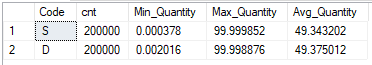
The things that stand out to me are that there are an equal number of supply and demand rows, both supply and demand have nearly the same average value, and the maximum quantity for both supply and demand is under 100. We can exploit the relatively low maximum quantity value to improve performance. A supply interval with a end point that is more than 100 units away from the demand end point cannot possibly intersect it. This is one of those things that feels intuitively correct, but I’ll go ahead and prove it anyway by contradiction.

Suppose that 100 is the maximum interval length, [d_start, d_end] and [s_start, s_end] overlap, s_end is more than 100 units away from d_end.

  1. The distance between end points implies that d_end < s_end – 100
  2. If they overlap, then s_start < d_end
  3. This implies that s_start < d_end < s_end – 100
  4. This implies that s_start < s_end – 100
  5. This implies that s_end – s_start > 100

The final statement is impossible because 100 is the maximum interval length. You can do the same proof in the other direction. Therefore, it should be safe to add some filters to our original query:

SELECT d.ID DemandId, s.ID as SupplyID,
CASE
WHEN d.IntervalEnd >= s.IntervalEnd THEN s.IntervalEnd - CASE WHEN s.IntervalStart >= d.IntervalStart THEN s.IntervalStart ELSE d.IntervalStart END
ELSE d.IntervalEnd - CASE WHEN s.IntervalStart >= d.IntervalStart THEN s.IntervalStart ELSE d.IntervalStart END
END TradeQuantity
FROM #demand_intervals d WITH (TABLOCK)
CROSS JOIN #supply_intervals s WITH (TABLOCK)
WHERE d.IntervalEnd > s.IntervalStart AND d.IntervalStart < s.IntervalEnd
AND s.IntervalEnd >= d.IntervalEnd - 100
AND s.IntervalEnd <= d.IntervalEnd + 100;

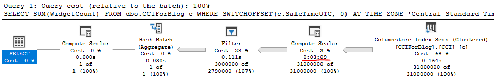
Now we can get a proper index seek on the s.IntervalEnd column. Performance is significantly better with this additional filter clause. The total runtimes for all steps, including the omitted temp table creation, are 1030 ms of CPU time and 345 ms of elapsed time. We are of course not using batch mode though:

Buckets

Time for more math. Starting with the following filter conditions:

AND s.IntervalEnd >= d.IntervalEnd – 100
AND s.IntervalEnd <= d.IntervalEnd + 100;

I can divide both sides by 100 and the condition will still be true:

AND s.IntervalEnd / 100 >= d.IntervalEnd / 100 – 1
AND s.IntervalEnd / 100 <= d.IntervalEnd / 100 + 1

You’ll have to take my word for it that the equation is still true if we truncate everything down to integers:

AND FLOOR(s.IntervalEnd / 100) >= FLOOR(d.IntervalEnd / 100) – 1
AND FLOOR(s.IntervalEnd / 100) <= FLOOR(d.IntervalEnd / 100) + 1

Now we’re dealing with integers, so we can express this as the following:

FLOOR(s.IntervalEnd / 100) IN (FLOOR(d.IntervalEnd / 100) – 1, FLOOR(d.IntervalEnd / 100) + 0, FLOOR(d.IntervalEnd / 100) + 1)

Rewriting once again:

FLOOR(s.IntervalEnd / 100) = FLOOR(d.IntervalEnd / 100) – 1
OR FLOOR(s.IntervalEnd / 100) = FLOOR(d.IntervalEnd / 100) + 0
OR FLOOR(s.IntervalEnd / 100) = FLOOR(d.IntervalEnd / 100) + 1

That’s still not eligible for a hash join, but it is if we change it to a UNION ALL:

... JOIN ON ...
FLOOR(s.IntervalEnd / 100) = FLOOR(d.IntervalEnd / 100) - 1

UNION ALL

... JOIN ON ...
FLOOR(s.IntervalEnd / 100) = FLOOR(d.IntervalEnd / 100) + 0

UNION ALL

... JOIN ON ...
FLOOR(s.IntervalEnd / 100) = FLOOR(d.IntervalEnd / 100) + 1

We have successfully transformed a single BETWEEN join filter into three joins with equality filters. All three of those joins are eligible for batch mode.

A visual representation may be helpful. Suppose we have two demand intervals that end in 150.2 and 298.2. We need to match those intervals with 8 supply intervals with end points that range from 1.1 to 399.1. To do so, we can divide the intervals into buckets of 100 width and join on matching bucket values as well as the immediately adjacent bucket values:

The demand interval that ends in 150.2 has a bucket value of 1, so it is matched with supply buckets 0, 1, and 2. In this way, we can guarantee that any supply interval that’s 100 or fewer units away ends up getting matched with the right demand intervals. The supply buckets with a background of red are only matched to the demand interval of 150.2, blue is only matched to the demand interval of 298.2, and purple is matched to both. The buckets are overly inclusive of course. The actual rows that might match based on distance have their font color changed in the same way, but filtering out extra rows later will be no problem. The important thing is that we have an equality condition to work with. Now that we can finally perform hash joins, it’s time to work out all of the details.

Gotta Go Fast

We need to perform three operations:

  1. Calculate the maximum interval length.
  2. Calculate running totals for supply and demand, their bucket values, and load them into temporary objects.
  3. Query the temp tables to load the final results into another table.

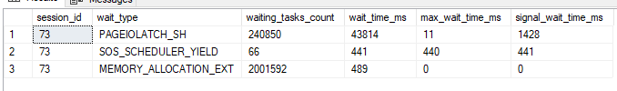
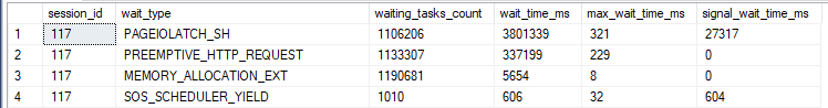
For step 1, we simply need an index on the Quantity column to make the query fast. We also need to get an exclusive lock and hold it until we’re finished with all of the steps. Otherwise the max length could change in the middle of our code’s execution.

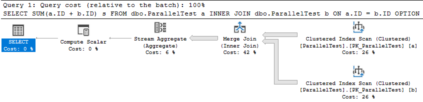
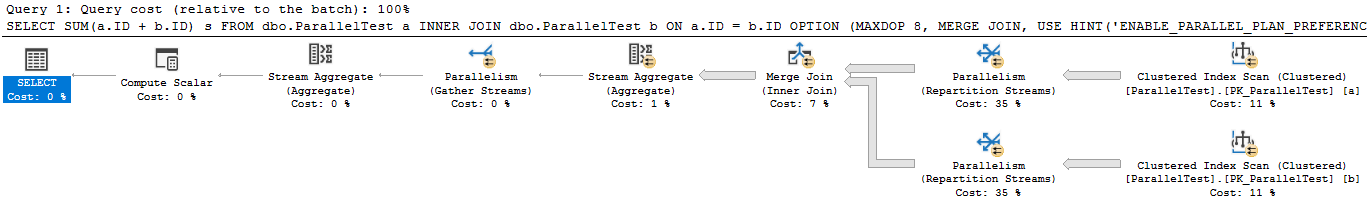
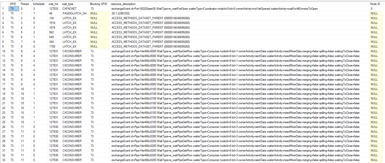
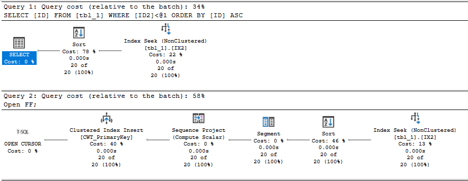
For step 2, the best performing options are either a MAXDOP 1 query with an ordered index scan and a batch mode window aggregate or a parallel query with a batch mode sort, parallel batch mode window aggregate, and parallel insert. An NCCI on the Auctions table is helpful in getting batch mode. In order to make the code go as fast as possible, I elected to use the parallel option at MAXDOP 4 even though it uses significantly more CPU time than the MAXDOP 1 option. DOP is at 4 instead of 8 due to contention caused by the NESTING_TRANSACTION_FULL latch. Here’s an estimated plan picture in case you don’t know what I mean by all of that:

For the third query, I’m using a UNION ALL of 3 joins that are eligible for batch mode like I said earlier. I added some query hints to reduce compile time.

As a step 0 that I forgot to mention earlier, create the following indexes on the Auctions table:

CREATE INDEX IX_Auctions__Code_ID__INCLUDE_Quantity ON Auctions (Code, ID) INCLUDE (Quantity);

CREATE INDEX IX_Auctions__Quantity ON Auctions (Quantity);

CREATE NONCLUSTERED COLUMNSTORE INDEX NCCI_Auctions ON Auctions (Code) with (MAXDOP = 1);

You can find the full code below for all three steps:

SET NOCOUNT ON;

DROP TABLE IF EXISTS #PairingsCursor2;
CREATE TABLE #PairingsCursor2
(
DemandID INT NOT NULL,
SupplyID INT NOT NULL,
TradeQuantity DECIMAL(19, 6) NOT NULL
);

DROP TABLE IF EXISTS #demand_intervals;
CREATE TABLE #demand_intervals (
ID INT NOT NULL,
IntervalStart DECIMAL(19, 6) NOT NULL,
IntervalEnd DECIMAL(19, 6) NOT NULL,
IntervalBucket BIGINT NOT NULL
);

DROP TABLE IF EXISTS #supply_intervals;
CREATE TABLE #supply_intervals (
ID INT NOT NULL,
IntervalStart DECIMAL(19, 6) NOT NULL,
IntervalEnd DECIMAL(19, 6) NOT NULL,
IntervalBucket BIGINT NOT NULL
);

DECLARE @MaxQuantityRange DECIMAL(19, 6);

BEGIN TRANSACTION;

SELECT @MaxQuantityRange = MAX(Quantity) - MIN(Quantity)
FROM Auctions WITH (TABLOCKX);

INSERT INTO #demand_intervals WITH (TABLOCK)
SELECT ID, rt - Quantity IntervalStart, rt IntervalEnd, CAST(rt / @MaxQuantityRange AS BIGINT) AS IntervalBucket
FROM
(
SELECT a.ID, Quantity, SUM(Quantity) OVER (ORDER BY a.ID ROWS BETWEEN UNBOUNDED PRECEDING AND CURRENT ROW) rt
FROM dbo.Auctions a WITH (TABLOCK)
WHERE Code = 'D'
) q
OPTION (USE HINT('ENABLE_PARALLEL_PLAN_PREFERENCE'), MAXDOP 4);

INSERT INTO #supply_intervals WITH (TABLOCK)
SELECT ID, rt - Quantity IntervalStart, rt IntervalEnd, CAST(rt / @MaxQuantityRange AS BIGINT) AS IntervalBucket
FROM
(
SELECT a.ID, Quantity, SUM(Quantity) OVER (ORDER BY a.ID ROWS BETWEEN UNBOUNDED PRECEDING AND CURRENT ROW) rt
FROM dbo.Auctions a WITH (TABLOCK)
WHERE Code = 'S'
) q
OPTION (USE HINT('ENABLE_PARALLEL_PLAN_PREFERENCE'), MAXDOP 4);

/*
-- prevents temp table caching, slight performance overhead in last query, but avoids "expensive" stats gathering for uncached object scenario
CREATE STATISTICS s0 ON #demand_intervals (IntervalBucket) WITH SAMPLE 0 ROWS;
CREATE STATISTICS s1 ON #supply_intervals (IntervalBucket) WITH SAMPLE 0 ROWS;
*/

INSERT INTO #PairingsCursor2 WITH (TABLOCK)
SELECT d.ID DemandId, s.ID as SupplyID,
CASE
WHEN d.IntervalEnd >= s.IntervalEnd THEN s.IntervalEnd - CASE WHEN s.IntervalStart >= d.IntervalStart THEN s.IntervalStart ELSE d.IntervalStart END
ELSE d.IntervalEnd - CASE WHEN s.IntervalStart >= d.IntervalStart THEN s.IntervalStart ELSE d.IntervalStart END
END TradeQuantity
FROM #demand_intervals d WITH (TABLOCK)
INNER JOIN #supply_intervals s WITH (TABLOCK) ON d.IntervalBucket = s.IntervalBucket
WHERE d.IntervalEnd > s.IntervalStart AND d.IntervalStart < s.IntervalEnd

UNION ALL

SELECT d.ID DemandId, s.ID as SupplyID, CASE WHEN d.IntervalEnd >= s.IntervalEnd THEN s.IntervalEnd - CASE WHEN s.IntervalStart >= d.IntervalStart THEN s.IntervalStart ELSE d.IntervalStart END
ELSE d.IntervalEnd - CASE WHEN s.IntervalStart >= d.IntervalStart THEN s.IntervalStart ELSE d.IntervalStart END
END TradeQuantity
FROM #demand_intervals d WITH (TABLOCK)
INNER JOIN #supply_intervals s WITH (TABLOCK) ON s.IntervalBucket = d.IntervalBucket - 1
WHERE d.IntervalEnd > s.IntervalStart AND d.IntervalStart < s.IntervalEnd

UNION ALL

SELECT d.ID DemandId, s.ID as SupplyID, CASE WHEN d.IntervalEnd >= s.IntervalEnd THEN s.IntervalEnd - CASE WHEN s.IntervalStart >= d.IntervalStart THEN s.IntervalStart ELSE d.IntervalStart END
ELSE d.IntervalEnd - CASE WHEN s.IntervalStart >= d.IntervalStart THEN s.IntervalStart ELSE d.IntervalStart END
END TradeQuantity
FROM #demand_intervals d WITH (TABLOCK)
INNER JOIN #supply_intervals s WITH (TABLOCK) ON s.IntervalBucket = d.IntervalBucket + 1
WHERE d.IntervalEnd > s.IntervalStart AND d.IntervalStart < s.IntervalEnd
OPTION (USE HINT('ENABLE_PARALLEL_PLAN_PREFERENCE'), MAXDOP 8, HASH JOIN, CONCAT UNION, FORCE ORDER, NO_PERFORMANCE_SPOOL); -- reduce compile time

COMMIT TRANSACTION;

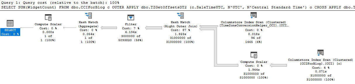
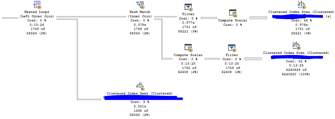
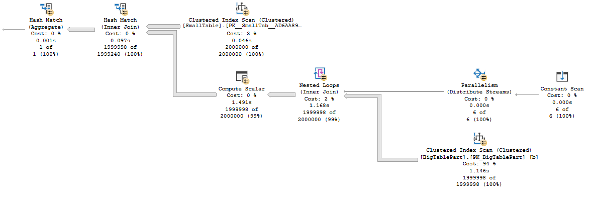
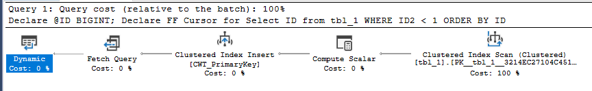
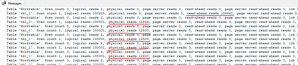
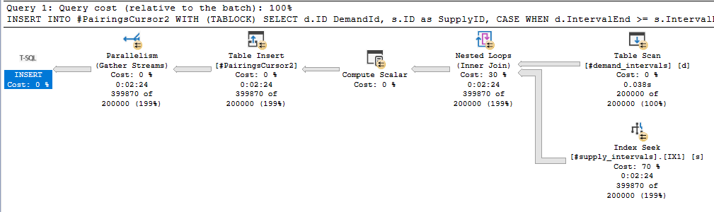
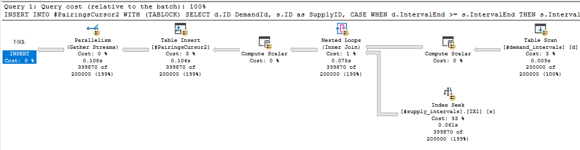
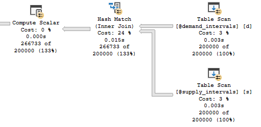
For the first execution, CPU time is generally around 1245 ms and elapsed time is around 500 ms. For subsequent executions, CPU time is around 634 ms and elapsed time is around 168 ms. Here is an actual execution plan for step 3:

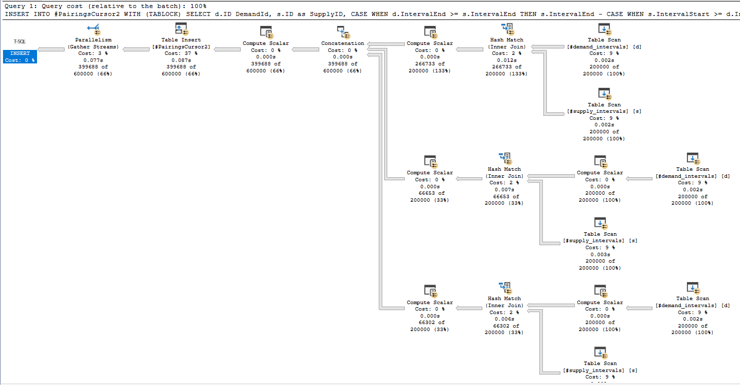
Not surprisingly, the join for matching buckets returns significantly more rows than the joins for adjacent buckets.

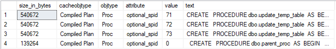
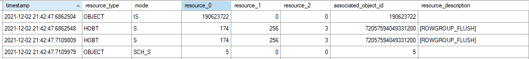
REEEEEEEEEEEEECOMPILES

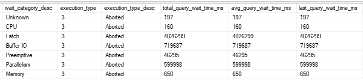
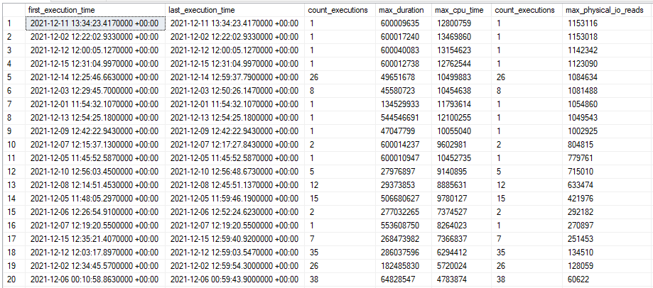
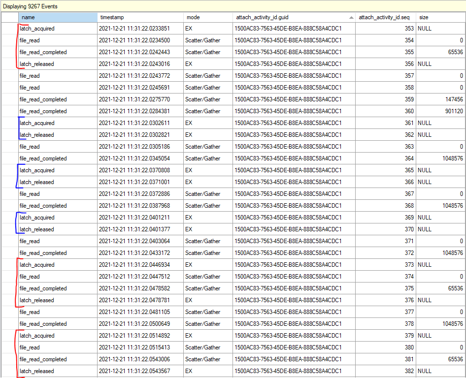
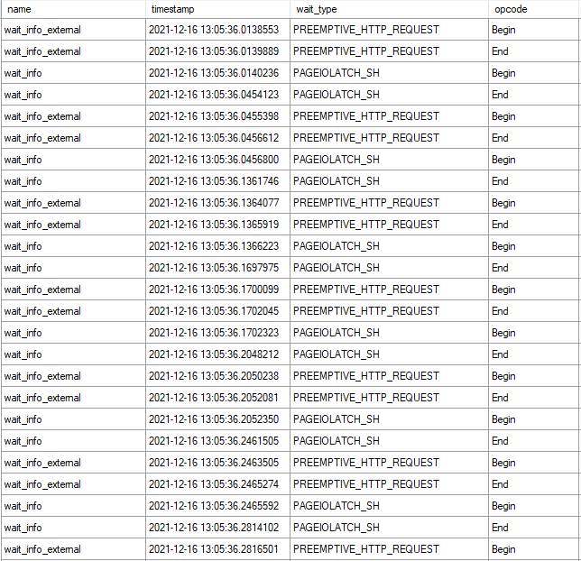
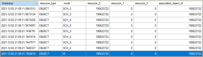
You may be wondering why the first execution takes so much longer than subsequent executions. The problem is the creation of temp table statistics. For some reason, SQL Server issues four StatMan queries per statistic that it creates:

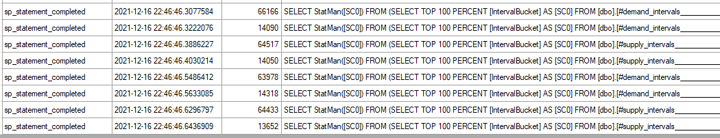
Some of them run at MAXDOP 1 and some of them run at MAXDOP 8 and all of that time adds up. After the first execution the creation of statistics no longer happens, I assume due to statistics caching for temporary tables. Even adding an explicit FULLSCAN create statistics statement doesn’t avoid this problem for some reason. You can create 0 row statistics if you like (see the commented out code), but I’m going to declare a moral victory here instead of digging into it further. If the biggest performance problem for your query is statistics creation on a pair of 200k row temp tables then you probably have pretty efficient code.

With that said, table variables are an interesting alternative here. I get consistent runtimes of 550 CPU ms and 230 ms of elapsed time using table variables. The deferred compilation feature introduced in SQL Server 2019 is important to get the right query plan. We lose a bit of runtime for the MAXDOP 1 table variable inserts and the final insert is slightly less efficient as well due to the missing statistics. Still, the runtimes are consistent between the first and second executions and overall CPU usage is down. Also you have to admit that seeing a batch mode table variable scan with a correct cardinality estimate (without RECOMPILE) is pretty cool:

Query Scaling

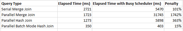
The performance of the batch mode query greatly depends on the maximum interval length. Query runtime increases in a roughly linear fashion as the max length increases:

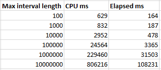
The linear pattern is broken for the final test case because all of the rows are in a single bucket at that point, so two out of three of the joins don’t do much of anything. Is this type of query safe to use in production? Sure, as long as you’re okay with significantly worse performance if a single outlier row happens to appear. Possible defenses against that include additional constraints on the data, knowing your data well, or writing a fallback algorithm if the maximum interval length is too long for the batch mode bucketizing approach to perform well.

Final Thoughts

This blog post shows how batch mode hash joins can be used as an efficient solution to find intersecting intervals, provided that the maximum interval length is sufficiently small. The important thing is everyone involved had fun. Thanks for reading!

Blocking on Columnstore Indexes that RCSI and NOLOCK Don’t Resolve

I recently ran into a production issue where a SELECT query that referenced a NOLOCK-hinted table was hitting a 30 second query timeout. Query store wait stats suggested that the issue was blocking on a table with a nonclustered columnstore index (NCCI). This was quite unexpected to me and I was eventually able to produce a reproduction of the issue. I believe this to be a bug in SQL Server that’s present in both RTM and the current CU as of this blog post (CU14). The issue also impacts CCIs as well but I did significantly less testing with that index type.

The Setup

First I’ll create a heap with 500k rows. All of the rows have the same value. I’ll also create an NCCI on the single column of the table.

DROP TABLE IF EXISTS dbo.TEST_NCCI_1;
CREATE TABLE dbo.TEST_NCCI_1 (
ID VARCHAR(10) NOT NULL
);

INSERT INTO dbo.TEST_NCCI_1
SELECT TOP (500000) '1'
FROM master..spt_values t1
CROSS JOIN master..spt_values t2;

CREATE NONCLUSTERED COLUMNSTORE INDEX NCCI ON dbo.TEST_NCCI_1 (ID) WITH (MAXDOP = 1);

The NCCI has a single compressed rowgroup with no rows in the delta store or delete buffer. It’s an honest table and I’m not trying to trick you:

We also need a table to join to. A heap with a single row will serve that need:

DROP TABLE IF EXISTS dbo.JOIN_TO_ME;
CREATE TABLE dbo.JOIN_TO_ME (
ID VARCHAR(10) NOT NULL
);

INSERT INTO dbo.JOIN_TO_ME VALUES ('1');

Suppose a different session has a long held exclusive table lock on TEST_NCCI_1. For example, the code below could be running in a different session with a yet to be committed transaction:

BEGIN TRANSACTION;

SELECT TOP (1) *
FROM dbo.TEST_NCCI_1 WITH (TABLOCKX);

Would you expect the following query to be blocked by the open transaction?

SELECT COUNT_BIG(*)
FROM dbo.TEST_NCCI_1 a WITH (NOLOCK)
Left Outer Join dbo.JOIN_TO_ME b WITH (NOLOCK) ON a.ID = b.ID;

Test Results

I ran 45 tests in total by varying the isolation level (SET TRANSACTION ISOLATION LEVEL) and the locking hint at the table level. You may be wondering why I bothered to do so. According to the documentation, a table level locking hint overrides the isolation level for read operations:

Only one of the isolation level options can be set at a time, and it remains set for that connection until it is explicitly changed. All read operations performed within the transaction operate under the rules for the specified isolation level unless a table hint in the FROM clause of a statement specifies different locking or versioning behavior for a table.

This is not what I observed which is part of why I believe that the current behavior in SQL Server should be considered a bug. In the table below, “YES” means that the query was blocked and “NO” means the query was able to execute. I used red font for the behavior which I believe to be in error based on my understanding of expected locking behavior in SQL Server.

To summarize the results:

  • The query is always blocked under the read committed, repeatable read, and serializable isolation levels. The table locking hint does not matter.
  • Blocking behavior works as expected under the read uncommitted and snapshot isolation levels.
  • RCSI does not help here. With RCSI, to avoid getting blocked you need to set the transaction isolation level to READ UNCOMMITTED.

I was able to use the lock_acquired extended event to see the problematic requested lock. In the screenshot below, the results are filtered to the object level. The first set of locks that occurred around the 11 second mark were under the read uncommitted isolation level. The second set of locks at around the 21 second mark where under the read committed isolation level. A table level NOLOCK hint was included for both queries.

To be clear, it is unexpected to see an IS object lock for a SELECT query with a table level NOLOCK hint. As far as I can tell, there are no interesting locks taken after the IS lock is acquired:

I attempted to investigate further by getting callstacks before the IS lock is acquired:

sqlmin.dll!XeSqlPkg::lock_acquired::Publish+0x228
sqlmin.dll!lck_lockInternal+0x1139
sqlmin.dll!LockAndCheckState+0x2c5
sqlmin.dll!GetHoBtLockInternal+0x445
sqlmin.dll!ColumnDataSetSession::WakeUp+0xa86
sqlmin.dll!NormalColumnDataSet::WakeUp+0xe
sqlmin.dll!ColumnDataSetSession::Create+0x183
sqlmin.dll!ColumnsetSS::WakeUpInternal+0x1ec
sqlmin.dll!ColumnsetSS::WakeUp+0x15e
sqlmin.dll!CreateDictionaryRowsetHelper+0x250
sqlmin.dll!CBpLocalDictionaryManager::GetSEStringDictionaryRowset+0x416
sqlmin.dll!CBpLocalDictionaryManager::FGetData+0xd1
sqlmin.dll!CBpDeepDataContextForBatch::GetStringValue+0x1d
sqlTsEs.dll!CTEsHashMultiData<167,1>::MdEsIntrinFn<CMDPureInput,CMDIteratorAllPureInputs>+0x13d
sqlTsEs.dll!CEsMDIntrinsicWrapper::UnaryImpl<&CTEsHashMultiData<167,1>::MdEsIntrinFn<CMDPureInput,CMDIteratorAllPureInputs>,&CTEsHashMultiData<167,1>::MdEsIntrinFn<CMDImpureInput,CMDIterator> >+0xd1
sqlTsEs.dll!CEsExecMultiData::GeneralEval+0x188
sqlTsEs.dll!CMultiDataEsRuntime::Eval+0x247
sqlmin.dll!CBpComputeMulticolumnHashRunTime::Eval+0x5b7
sqlmin.dll!CBpPartialJoin::ProcessProbeSide+0x445
sqlmin.dll!CBpQScanHashJoin::Main+0x148
sqlmin.dll!CBpQScanHashJoin::BpGetNextBatch+0x28
sqlmin.dll!CBpQScan::GetNextBatch+0x6f
sqlmin.dll!CBpChildIteratorScanner::BpGetNextBatch+0x12
sqlmin.dll!CBpQScanHashAggNew::ProcessInput+0x8b

I’m not terribly surprised to see a reference to a dictionary in the callstacks because I’m not able to reproduce the issue with an INT or BIGINT column. However, I have no idea where to go from here.

Workarounds

Adding an IGNORE_NONCLUSTERED_COLUMNSTORE_INDEX query hint was an effective workaround for all of my test cases. I experienced the expected locking behavior for all test cases with that hint, so it is apparent to me that the issue is caused by the query plan reading from the NCCI.

Disabling batch mode using the DISALLOW_BATCH_MODE use hint seems to be an effective workaround as well, but I did not test this as thoroughly.

Changing the isolation level may also be an acceptable way to avoid the unexpected blocking for some scenarios. For example, if you already have a NOLOCK table hint in place then changing the transaction isolation level to read uncommitted may not introduce any new data correctness issues.

Final Thoughts

For some queries, a simple join on a VARCHAR column between a table with a columnstore index and another table can lead to unexpected blocking, even with a table level NOLOCK hint or with read committed snapshot isolation enabled for the database. This is frustrating and disappointing behavior from a concurrency perspective. It is an odd scenario where enabling snapshot isolation offers a significant benefit over enabling read committed snapshot isolation. I hope that this locking behavior changes in a future version of SQL Server. Thanks for reading!

Why does FAST_FORWARD make some cursors so much faster in SQL Server?

If you’re like me, you started your database journey by defining cursors with the default options. This went on until a senior developer or DBA kindly pointed out that you can get better performance by using the FAST_FORWARD option. Or maybe you were a real go-getter and found Aaron Bertrand’s performance benchmarking blog post on different cursor options. I admit that for many years I didn’t care to know why FAST_FORWARD sometimes made my queries faster. It had “FAST” in the name and that was good enough for me.

Recently I saw a production issue where using the right cursor options led to a 1000X performance improvement. I decided that ten years of ignorance was enough and finally did some research on different cursor options. This post contains a reproduction and discussion of the production issue.

A Dramatic Example

The code below creates a 16 GB table. It has a primary key and clustered index on the ID column and a nonclustered index on the ID2 column. You can adjust the TOP value to insert fewer rows if you wish to create a smaller table, but don’t drop it below 200000.

DROP TABLE IF EXISTS tbl_1;

CREATE TABLE tbl_1 (
ID BIGINT NOT NULL,
ID2 BIGINT NOT NULL,
PAGE_FILLER VARCHAR(5000) NOT NULL,
PRIMARY KEY (ID)
);

INSERT INTO tbl_1 WITH (TABLOCK)
SELECT RN, RN % 100000, REPLICATE('Z', 5000)
FROM
(
	SELECT TOP (2000000) ROW_NUMBER() OVER (ORDER BY (SELECT NULL)) RN
	FROM master..spt_values t1
	CROSS JOIN master..spt_values t2
) q
OPTION (MAXDOP 1);

CREATE INDEX IX2 ON tbl_1 (ID2);

Consider the following select query, which is a simplified example of the production query:

Select ID
from tbl_1
WHERE ID2 < 1
ORDER BY ID;

There’s an index on ID2 and the filter is highly selective: only 20 rows out of 2 million will match. I would expect the query optimizer to use that index and for the query to finish instantly. The following stored procedure defines a FAST_FORWARD cursor for that SELECT query, fetches the 20 matching rows, and does nothing with them:

CREATE OR ALTER PROCEDURE CURSOR_WITH_FF
AS
BEGIN
SET NOCOUNT ON;

Declare @ID BIGINT;

Declare FF Cursor FAST_FORWARD for
Select ID
from tbl_1
WHERE ID2 < 1
ORDER BY ID;

Open FF;
Fetch Next from FF into @ID;
WHILE @@FETCH_STATUS = 0
BEGIN
	Fetch Next from FF into @ID;
END;
Close FF;
Deallocate FF;
END;

Executing the stored procedure takes about 2 ms on my machine. In this case, I get a query plan that’s very similar to what I’d get by running a simple SELECT query. There’s some additional cursor garbage, but that doesn’t impact performance in this case:

SQL Server Query Plan

Regrettably, the code takes 50 seconds to execute on my machine if I remove the FAST_FORWARD option. What is responsible for the dramatic difference in runtime?

The “What”

We can start by looking at the query plan for the default cursor:

SQL Server Query Plan

The query optimizer decided to do an ordered clustered index scan instead of using the IX2 index. We’re getting all rows from the cursor so we have to read through the whole table. That’s 20 scans with each scan covering about 5% of the table. We should definitely expect this to be less efficient than the FAST_FORWARD plan, but a 50 second execution time felt too slow based on what I know about my hardware. Looking at the wait stats:

SQL Server Query Plan

It’s certainly not surprising that I/O is the biggest contributor to wait time (what else would it be?), but why do I have so much I/O wait time when I have fast, locally attached storage with an average latency less than 1 ms? For a comparison test, I decided to force the query plan that the cursor picks but to run it outside of the cursor. The following code finished in about 8 seconds on my machine:

CHECKPOINT;
DBCC DROPCLEANBUFFERS;

Select ID
from tbl_1 WITH (INDEX(1))
WHERE ID2 < 1
ORDER BY ID
OPTION (MAXDOP 1);

Using sys.dm_io_virtual_file_stats, I found that the cursor was doing about 240000 I/Os with an average I/O size of 66 KB. The single SELECT query did about 10000 I/Os with an average I/O size of 1.7 MB. The key difference is that only the first query execution of the cursor is able to get read-ahead reads:

SQL Server Query Plan

For the cursor execution, we don’t get read ahead reads for 95% of the I/O needed for the query. Even a sub-ms I/O latency can be painful when you have to do 240000 I/Os with a DOP 1 query. In summary, the FAST_FORWARD cursor is able to use an index to efficiently seek to the 20 matching rows. The cursor with default options does about 15 GB of I/O that’s not eligible for read-ahead reads.

Of course, the situation should be expected to be much worse in the cloud. Using the quoted latency of 5-10 ms for general purpose Managed Instances, one might expect the cursor with default options to take between 20 and 40 minutes. Just for fun, I decided to test it against a 4 vCore Managed Instance. The cursor with the FAST_FORWARD option took about 120 ms. The cursor with default options took about 70 minutes. Here are the wait stats for the execution:

SQL Server Query Plan

To put a positive spin on it: using the correct cursor options improved performance by 35000X on the Managed Instance.

The “Why”

I’ll start by saying that I don’t want to be a cursor expert. I’d much rather be an expert in not using cursors. I was having a lot of trouble explaining why the default cursor was getting such a bad query plan, but fortunately I was scooped 12 years ago. I’m going to reproduce the entire section on dynamic plans because you never know when a Microsoft hosted blog post will disappear:

A dynamic plan can be processed incrementally. In SQL Server we do this by serializing the state of the query execution into what we call a marker. Later, we can build a new query execution tree, use the marker to reposition each operator. Moreover, a dynamic plan can move forwards and backwards relative to its current position. Dynamic plans are used by both dynamic and some fast_forward cursors.

A dynamic plan consists only of dynamic operators — operators that support markers and moving forwards and backwards. This corresponds closely, but not exactly, to the query processing notion of streaming operators (vs. stop-and-go). But not every streaming operator is dynamic. In SQL Server, dynamic means:

1. The operator can be repositioned to its current position using a marker, or to a relative position (either next or previous) from its current one.

2. The operator’s state has to be small, so the marker can be small. No row data can be stored in the operator. In particular, no sort table, hash table, or work table. Not even one row can be stored, since a single row can be very large.

Without a dynamic plan, the cursor would need temporary storage to keep the query result set (or keyset thereof). A dynamic plan does no such thing! However, certain operators are disqualified — hash join, hash agg, compute sequence, and sort, for example. This leads to sub-optimal plans.

In short, you can consider a dynamic plan to be similar in concept to a plan with no blocking operators, but there are some additional restrictions. Reliable sources tell me that a cursor with default options will always pick a dynamic plan if one is available. For our SELECT query, a dynamic plan is indeed available. The ordering of the clustered index can be used to return sorted rows without doing an explicit sort. The IX2 index cannot be used for ordering because I’m filtering on ID2 with an inequality. Changing the query to do an equality filter instead allows for a dynamic plan that uses the IX2 index:

SQL Server Query Plan

What about cursors without default options? Going back to the original query, specifying the STATIC or KEYSET option avoids the bad query plan and uses the IX2 index to do an index seek. Both of those options write the cursor result set to a table in tempdb, so it makes intuitive sense that there wouldn’t be some kind of restriction that forces a clustered index scan.

Specifying the FAST_FORWARD option allows the query optimizer to pick between a static and dynamic plan. In this case, the static plan is obviously much more efficient, and the query optimizer is aware of that. It picks the static plan that doesn’t do the clustered index scan.

For completeness, specifying the READ_ONLY option also results in the index seek, as long as the DYNAMIC option isn’t also specified.

In general, I would say that FAST_FORWARD is still a good starting point for your cursors as long as your application code allows for the restrictions that come with it. FAST_FORWARD alone isn’t always sufficient to get query performance that is similar to what you’d get with a standard SELECT. As Erik points out, you’ll end up with a MAXDOP 1 query with that option. The query optimizer may also choose a worse dynamic plan instead of a static plan if the estimated query plan costs don’t reflect reality. Using STATIC instead of FAST_FORWARD can be quite helpful in some cases, but you’ll have to test your cursor specifically to know for sure. Of course, you may be able to write your code without using a cursor instead.

Insufficient Permissions

As someone always on the lookout for cool demos, this bit of the documentation caught my eye:

If a DECLARE CURSOR using Transact-SQL syntax does not specify READ_ONLY, OPTIMISTIC, or SCROLL_LOCKS, the default is as follows:

If the SELECT statement does not support updates (insufficient permissions, accessing remote tables that do not support updates, and so on), the cursor is READ_ONLY.

Could I get better performance by running the code as a login with less privileges? Sadly, I couldn’t get this to work. I verified that the lowly ‘erik’ login couldn’t modify data in the table but I got the same query plan as before. There was also no change in the properties column from the sys.dm_exec_cursors DMF.

I don’t know if the documentation was wrong or if I was doing something wrong on my end. I’d be interested in seeing a working repro of this if anyone has one.

Final Thoughts

Some query patterns can experience extremely poor performance with the default cursor options. You may be able to identify these queries by sorting by total logical reads in the standard SSMS query store reports. In our production environment we had a few cursors that were doing far more logical reads than anything else on the database, so they were easy to pick out. We were able to significantly speed up some of those queries just by adding the FAST_FORWARD option.

Thanks for reading!

Going Further


If this is the kind of SQL Server stuff you love learning about, you’ll love my training. I’m offering a 75% discount to my blog readers if you click from here. I’m also available for consulting if you just don’t have time for that and need to solve performance problems quickly.