Lots of smart people have written about join containment, but none of the explanations really made sense to me. I felt like a student memorizing definitions for a test. Sure, I could tell you the definitions of base and simple containment, but what practical difference does it make when it comes to cardinality estimation? The concept finally clicked when working on an Oracle query of all things, and as a result I wrote this blog post. All testing was done on SQL Server 2017 with a CE version of 140.
A Note on Join Cardinality
Join cardinality calculations are incredibly complex in SQL Server. You can get a small taste of that complexity here. I’ve chosen the example data in this blog post to avoid most of the complexity. The formulas and concepts described in this post can’t be used to model join cardinality generally, but I hope that they serve as a good illustration of containment.
Demo Tables
All of the demo tables have identical structures with similar data. The first column, UNIQUE_ID, stores unique integers in the range specified in the table name. For example, TA_1_TO_1000000 is a table that stores integers from 1 to 1000000. The second column, MOD_FILTER, stores integers from 1 to 100 cycling through all rows. The purpose of this column is to make filtering cardinality estimates simple to calculate and predict. For example, MOD_FILTER BETWEEN 1 AND 50 will return 50% of the rows from the table. Full statistics are gathered on all columns, and there are four tables in all.
DROP TABLE IF EXISTS dbo.TA_1_TO_1000000;

CREATE TABLE dbo.TA_1_TO_1000000 (
	UNIQUE_ID BIGINT NOT NULL,
	MOD_FILTER BIGINT NOT NULL
);

INSERT INTO dbo.TA_1_TO_1000000
	WITH (TABLOCK)
SELECT t.RN
, 1 + t.RN % 100
FROM
(
	SELECT TOP (1000000) ROW_NUMBER()
		OVER (ORDER BY (SELECT NULL)) RN
	FROM master..spt_values t1
	CROSS JOIN master..spt_values t2
) t
OPTION (MAXDOP 1);

CREATE STATISTICS S1 ON dbo.TA_1_TO_1000000 (UNIQUE_ID)
	WITH FULLSCAN;
CREATE STATISTICS S2 ON dbo.TA_1_TO_1000000 (MOD_FILTER)
	WITH FULLSCAN;

DROP TABLE IF EXISTS dbo.TB_1_TO_1000000;

CREATE TABLE dbo.TB_1_TO_1000000 (
	UNIQUE_ID BIGINT NOT NULL,
	MOD_FILTER BIGINT NOT NULL
);

INSERT INTO dbo.TB_1_TO_1000000
	WITH (TABLOCK)
SELECT t.RN
, 1 + t.RN % 100
FROM
(
	SELECT TOP (1000000) ROW_NUMBER()
		OVER (ORDER BY (SELECT NULL)) RN
	FROM master..spt_values t1
	CROSS JOIN master..spt_values t2
) t
OPTION (MAXDOP 1);

CREATE STATISTICS S1 ON dbo.TB_1_TO_1000000 (UNIQUE_ID)
	WITH FULLSCAN;
CREATE STATISTICS S2 ON dbo.TB_1_TO_1000000 (MOD_FILTER)
	WITH FULLSCAN;

DROP TABLE IF EXISTS dbo.TC_1_TO_100000;

CREATE TABLE dbo.TC_1_TO_100000 (
	UNIQUE_ID BIGINT NOT NULL,
	MOD_FILTER BIGINT NOT NULL
);

INSERT INTO dbo.TC_1_TO_100000
	WITH (TABLOCK)
SELECT t.RN
, 1 + t.RN % 100
FROM
(
	SELECT TOP (100000) ROW_NUMBER()
		OVER (ORDER BY (SELECT NULL)) RN
	FROM master..spt_values t1
	CROSS JOIN master..spt_values t2
) t
OPTION (MAXDOP 1);

CREATE STATISTICS S1 ON dbo.TC_1_TO_100000 (UNIQUE_ID)
	WITH FULLSCAN;
CREATE STATISTICS S2 ON dbo.TC_1_TO_100000 (MOD_FILTER)
	WITH FULLSCAN;

DROP TABLE IF EXISTS dbo.TD_500001_TO_1500000;

CREATE TABLE dbo.TD_500001_TO_1500000 (
	UNIQUE_ID BIGINT NOT NULL,
	MOD_FILTER BIGINT NOT NULL
);

INSERT INTO dbo.TD_500001_TO_1500000
	WITH (TABLOCK)
SELECT t.RN
, 1 + t.RN % 100
FROM
(
	SELECT TOP (1000000) 500000 + ROW_NUMBER()
		OVER (ORDER BY (SELECT NULL)) RN
	FROM master..spt_values t1
	CROSS JOIN master..spt_values t2
) t
OPTION (MAXDOP 1);

CREATE STATISTICS S1 ON dbo.TD_500001_TO_1500000 (UNIQUE_ID)
	WITH FULLSCAN;
CREATE STATISTICS S2 ON dbo.TD_500001_TO_1500000 (MOD_FILTER)
	WITH FULLSCAN;
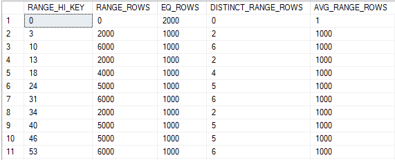
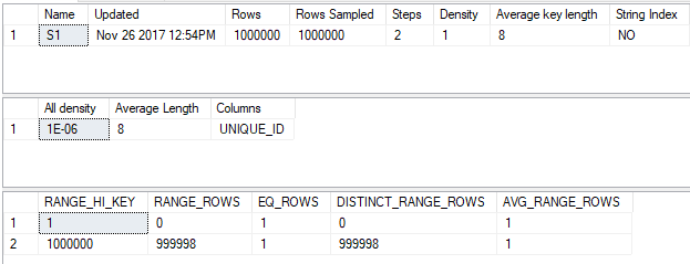
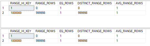
The statistics objects are perfect in that they fully describe the data. Here’s the statistics output for the UNIQUE_ID column:
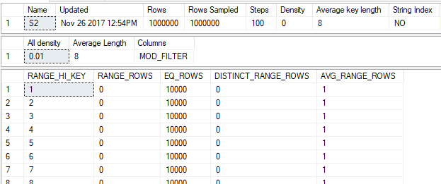
And here’s the output for the MOD_FILTER column:
This only happened because the table was populated with very simple data that fits well within the framework for generating histograms in SQL Server. Gathering statistics, even with FULLSCAN, will often not perfectly represent the data in the column.
A Simple Model of Join Cardinality Estimation
Consider the following simple query:
SELECT *
FROM TB_1_TO_1000000 b
INNER JOIN dbo.TD_500001_TO_1500000 d
	ON b.UNIQUE_ID = d.UNIQUE_ID;
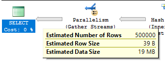
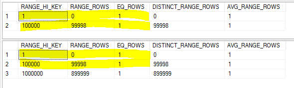
We know that exactly 500000 rows will be returned, but how might SQL Server estimate the number of rows to be returned? Let’s look at the histograms and try to align their steps:
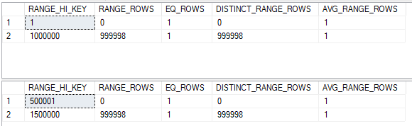
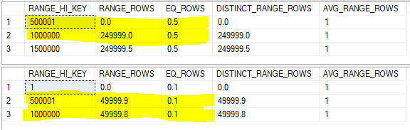
That doesn’t exactly work, but we can split up the histogram steps so they align. The assumption of uniformity within the step isn’t even needed here because we know that there aren’t missing any integer values. The histograms below are equivalent to the original ones:
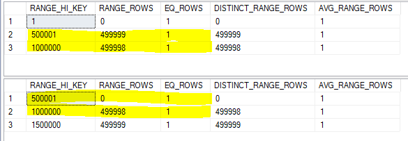
Now the RANGE_HI_KEY values align. For the step with a high value of 500001 we can expect only one row to match between tables. For the step with a high value of 1000000 we can expect 499998 + 1 rows to match. This brings the total row estimate to 500000, which happens to match what I get in SQL Server 2017 with the new CE. Remember, what we’re doing here isn’t how the query optimizer does the calculation. This is just a simple model that will be useful later.
Now consider the two queries below:
SELECT *
FROM TA_1_TO_1000000 a
INNER JOIN dbo.TB_1_TO_1000000 b
	ON a.UNIQUE_ID = b.UNIQUE_ID
WHERE a.MOD_FILTER BETWEEN 1 AND 50
AND b.MOD_FILTER BETWEEN 1 AND 50;

SELECT *
FROM TA_1_TO_1000000 a
INNER JOIN dbo.TB_1_TO_1000000 b
	ON a.UNIQUE_ID = b.UNIQUE_ID
WHERE a.MOD_FILTER BETWEEN 1 AND 50
AND b.MOD_FILTER BETWEEN 51 AND 100;
We know that the first query will return 500k rows and the second query will return 0 rows. However, can SQL Server know that? Each statistics object only contains information about its own column. There’s no correlation between the UNIQUE_ID and MOD_FILTER columns, so there isn’t a way for SQL Server to know that the queries will return different estimates. The query optimizer can create an estimate based on the filters on the WHERE clause and on the histograms of the join columns, but there’s no foolproof way to do that calculation. The presence of the filters introduces uncertainty into the estimate, even with statistics that perfectly describe the data for each column. The containment assumption is all about the modeling assumption that SQL Server has to make to resolve that uncertainty.
Base Containment
Base containment is the assumption that the filter predicates are independent from the join selectivity. The estimate for the join should be obtained by multiplying together the selectivity from both filters and the join. The query optimizer uses base containment starting with CE model version 120, also known as the new CE introduced in SQL Server 2014. It can be used with the legacy CE if trace flag 2301 is turned on. The best reference for trace flag 2301 is a blog post from 2006 which is no longer published.
Let’s go back to this example query:
SELECT *
FROM TA_1_TO_1000000 a
INNER JOIN dbo.TB_1_TO_1000000 b
	ON a.UNIQUE_ID = b.UNIQUE_ID
WHERE a.MOD_FILTER BETWEEN 1 AND 50
AND b.MOD_FILTER BETWEEN 1 AND 50;
The selectivity for the filter on MOD_FILTER is 0.5 for both tables. This is because there are 100 unique values for MOD_FILTER between 1 and 100 and each value matches 1% of the table. We can see this by getting an estimated query plan on just TA_1_TO_1000000:
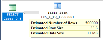
The table has 1 million rows, so the estimate is 500000 = 0.5 * 1000000.
That leaves the join selectivity. We put the same data into both tables:
We don’t need highlighters to see that the join selectivity is 1.0.
Putting it all together, the cardinality estimate under base containment for this query should be 1000000 * 1.0 * 0.5 * 0.5 = 250000. This is indeed the estimate:
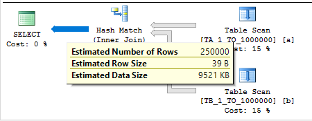
Of course, this doesn’t match the actual number of rows which is 500000. But it’s easy to change the filter predicates so that the estimated number of rows and the actual number of rows match.
Simple Containment
Simple containment is the assumption that the filter predicates are not independent. The estimate for the join should be obtained by applying the filter selectivities to the join histograms and joining based on the adjusted histograms. The query optimizer uses simple containment within the legacy CE. Simple containment can be used in the new CE via trace flag or USE HINT.
Let’s go back to the same example query:
SELECT *
FROM TA_1_TO_1000000 a
INNER JOIN dbo.TB_1_TO_1000000 b
	ON a.UNIQUE_ID = b.UNIQUE_ID
WHERE a.MOD_FILTER BETWEEN 1 AND 50
AND b.MOD_FILTER BETWEEN 1 AND 50
OPTION (
USE HINT ('ASSUME_JOIN_PREDICATE_DEPENDS_ON_FILTERS')
);
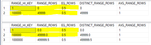
We know that the filter selectivity for both tables is 0.5. How can that be used to adjust the histograms? The simplest method would be to just multiply RANGE_ROWS, EQ_ROWS, and DISTINCT_RANGE_ROWS by the filter selectivity. After doing so we’re left with two still identical histograms:
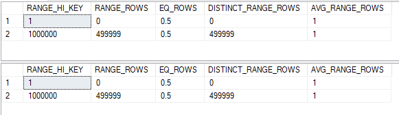
It might seem odd to work with fractions of a row, but as long as everything is rounded at the end why should it matter? With two identical, aligned histograms it seems reasonable to expect a cardinality estimate of 0.5 + 499999 + 0.5 = 500000. This is exactly what we get in SQL Server:
The actual row estimate matches the estimated row estimate because the filters are perfectly correlated. Every row left after filtering still has a matching row in the other table.
Just One Filter
What happens if we filter on just a single table? For example:
SELECT *
FROM dbo.TA_1_TO_1000000 a
INNER JOIN dbo.TB_1_TO_1000000 b
	ON a.UNIQUE_ID = b.UNIQUE_ID
WHERE a.MOD_FILTER BETWEEN 1 AND 30;

SELECT *
FROM dbo.TA_1_TO_1000000 a
INNER JOIN dbo.TB_1_TO_1000000 b
	ON a.UNIQUE_ID = b.UNIQUE_ID
WHERE a.MOD_FILTER BETWEEN 1 AND 30
OPTION (
USE HINT ('ASSUME_JOIN_PREDICATE_DEPENDS_ON_FILTERS')
);
For base containment, we know that the filter selectivity is 0.3 and the join selectivity is 1.0. We can expect a cardinality estimate of 1000000 * 1.0 * 0.3 = 300000 rows.
For simple containment we need to multiply the histogram for TA_1_TO_1000000 by 0.3. Here’s what the two histograms look like after factoring in filter selectivity:
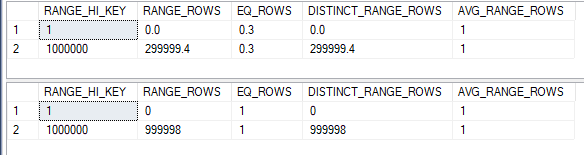
What should the estimate be? One approach would be to assume that everything matches between the aligned steps. So we end up with 0.3 rows from the step with a RANGE_HI_KEY of 1 and 299999.4 + 0.3 rows from the step with a RANGE_HI_KEY of 1000000. The combined estimate is 300000 rows, which matches the base containment estimate. Why shouldn’t they match? Without filters on both tables there’s no concept of correlation. If it helps you can imagine a filter of 1 = 1 on TB_1_TO_1000000. For base containment multiplying by 1.0 won’t change the estimate and for simple containment multiplying by 1 won’t change the histogram. That just leaves a single filter selectivity of 0.3 for TA_1_TO_1000000 and both estimates should be the same.
For both queries the estimated number of rows in SQL Server is 300000. Our calculations match the SQL Server query optimizer exactly for this query.
Filtering on the Join Column
What happens if we filter on the join columns of both tables? For example:
SELECT *
FROM dbo.TA_1_TO_1000000 a
INNER JOIN dbo.TB_1_TO_1000000 b
	ON a.UNIQUE_ID = b.UNIQUE_ID
WHERE a.UNIQUE_ID BETWEEN 1 AND 200000
AND b.UNIQUE_ID BETWEEN 1 AND 200000;

SELECT *
FROM dbo.TA_1_TO_1000000 a
INNER JOIN dbo.TB_1_TO_1000000 b
	ON a.UNIQUE_ID = b.UNIQUE_ID
WHERE a.UNIQUE_ID BETWEEN 1 AND 200000
AND b.UNIQUE_ID BETWEEN 1 AND 200000
OPTION (
USE HINT ('ASSUME_JOIN_PREDICATE_DEPENDS_ON_FILTERS')
);
Think back to why we need containment in the first place. When there are filters on columns that aren’t the join columns then we need to make an assumption as to how the selectivities all interact with each other. With a filter on the join column we can just adjust the histogram of the join column directly. There isn’t any uncertainty. Here’s what the histograms could look like:
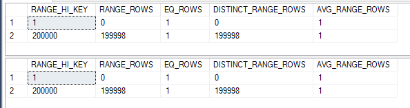
In which case, it seems obvious that the final estimate should be 200000 rows. Simple containment does not result in a different estimate here.
Removing Rows
So far the examples have been very simple. We’ve joined tables that contain the exact same data. What if one table has fewer rows than the other table? Consider the following pair of queries:
SELECT *
FROM dbo.TC_1_TO_100000 c
INNER JOIN dbo.TB_1_TO_1000000 b
	ON c.UNIQUE_ID = b.UNIQUE_ID
WHERE c.MOD_FILTER BETWEEN 1 AND 50
AND b.MOD_FILTER BETWEEN 1 AND 50;

SELECT *
FROM dbo.TC_1_TO_100000 c
INNER JOIN dbo.TB_1_TO_1000000 b
	ON c.UNIQUE_ID = b.UNIQUE_ID
WHERE c.MOD_FILTER BETWEEN 1 AND 50
AND b.MOD_FILTER BETWEEN 1 AND 50
OPTION (
USE HINT ('ASSUME_JOIN_PREDICATE_DEPENDS_ON_FILTERS')
);
It’s important to call out here that TC_1_TO_100000 has just 100000 rows instead of one million. For base containment, we know that the selectivity will be 0.5 for both tables. What about join selectivity? The histogram steps of course aren’t aligned:
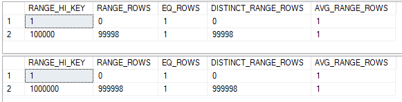
The data is densely packed, so we can use the same trick as before to split the histogram for the larger table:
Every row in histogram for the smaller table has a match in the histogram of the larger table. From the point of view of the smaller table the join selectivity is 1.0. Multiplying together all three selectivities gives a final row estimate of 100000 * 1.0 * 0.5 * 0.5 = 25000. This matches the row estimate within SQL Server exactly.
For simple containment we need to apply the filter selectivities of 0.5 to both tables. We also need to align the histograms by splitting the larger histogram. Both will be done in one step:
Every row in the smaller histogram once again matches. Our final estimate is 0.5 + 49999 + 0.5 = 50000 which exactly matches the SQL Server query optimizer.
Unmatched Rows
What happens if the tables have the same number of rows but they clearly don’t contain the same data? Consider the following pair of queries:
SELECT *
FROM dbo.TD_500001_TO_1500000 d
INNER JOIN dbo.TB_1_TO_1000000 b
	ON d.UNIQUE_ID = b.UNIQUE_ID
WHERE d.MOD_FILTER BETWEEN 1 AND 50
AND b.MOD_FILTER BETWEEN 1 AND 10;

SELECT *
FROM dbo.TD_500001_TO_1500000 d
INNER JOIN dbo.TB_1_TO_1000000 b
	ON d.UNIQUE_ID = b.UNIQUE_ID
WHERE d.MOD_FILTER BETWEEN 1 AND 50
AND b.MOD_FILTER BETWEEN 1 AND 10
OPTION (
USE HINT ('ASSUME_JOIN_PREDICATE_DEPENDS_ON_FILTERS')
);
The filter predicate for TB_1_TO_1000000 is 0.1 and the filter predicate for TD_500001_TO_1500000 is 0.5. Here are our starting histograms:
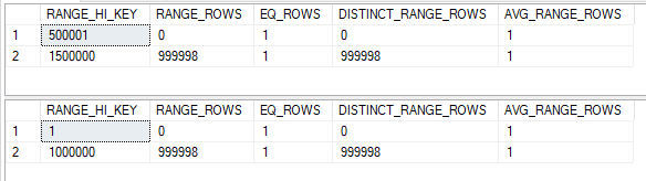
The little man who lives inside the cardinality estimator needs to slice them up so they align. His work is complete:
The top histogram has 500000 unmatched rows in the step with a RANGE_HI_KEY of 1500000, so the join selectivity is 500000 / 1000000 = 0.5. Putting all three selectivities together, the cardinality estimate with base containment should be 1000000 * 0.5 * 0.1 * 0.5 = 25000. This exactly matches SQL Server.
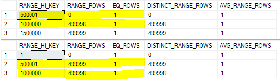
You know the drill for simple containment. We need to multiply each sliced histogram by its filter selectivity:
That’s pretty messy. I’m going to assume that every row has a match between the two shared steps, so the estimate should be 0.1 + 49999.8 + 0.1 = 50000. The number of estimated rows reported by SQL Server is 50000.4 :
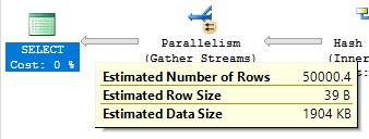
What happened? Did the little man only measure once before cutting? This is one of those examples where there’s other complicated stuff going on under the hood, so the predicted row estimate doesn’t match up exactly. Interestingly, the estimate with the legacy cardinality estimator is exactly 50000.
An Approximate Formula
- Define
T1_CARDINALITY as the number of rows in the first joined table.
- Define
T1_FILTER_SELECTIVITY as the filter selectivity of the filter predicates of the first table. This number ranges from 0.0 to 1.0, with 1.0 for filters that remove no rows.
- Define
T2_CARDINALITY as the number of rows in the second joined table.
- Define
T2_FILTER_SELECTIVITY as the filter selectivity of the filter predicates of the second table. This number ranges from 0.0 to 1.0, with 1.0 for filters that remove no rows.
- Define
JOIN_SELECTIVITY as the selectivity of the two histograms of the joined columns from the point of view of the smaller table. This number ranges from 0.0 to 1.0, with 1.0 meaning that all rows in the smaller table have a match in the larger table.
Based on the tests above, we can model the cardinality estimates for base and simple containment as follows:
Base containment = JOIN_SELECTIVITY * LEAST(T1_CARDINALITY, T2_CARDINALITY) * T1_FILTER_SELECTIVITY * T2_FILTER_SELECTIVITY
Simple containment = JOIN_SELECTIVITY * LEAST(T1_FILTER_SELECTIVITY * T1_CARDINALITY, T2_FILTER_SELECTIVITY * T2_CARDINALITY)
Remember that this isn’t how SQL Server actually does it. However, I think that it shows the difference between base containment and simple containment quite well. For simple containment the filters are applied to the histograms and for base containment all of the selectivities are independent.
A Mathematical Proof?
So far simple containment has always had a higher cardinality estimate than base containment. Looking at the formulas it certainly feels like simple should have a higher estimate. Can we prove that the estimate will always be higher using the above formulas? It’s been quite a few years so I apologize for the proof below, but I believe that it gets the job done.
Definitions:
JS = JOIN_SELECTIVITY
C1 = T1_CARDINALITY
F1 = T1_FILTER_SELECTIVITY
C2 = T2_CARDINALITY
F2 = T2_FILTER_SELECTIVITY
Attempt a proof by contradiction, so assume the opposite of what we want to prove:
JS * LEAST(C1, C2) * F1 * F2 > JS * LEAST(F1 * C1, F2 * C2)
We know that JS > 0, F1 > 0, and F2 > 0, so:
LEAST(C1, C2) > LEAST(C1 / F2, C2 / F1)
The left hand expression can only evalute to C1 or C2. Let’s assume that it evaluates to C1, so C1 <= C2. We know that F1 <= 1, so C2 <= C2 / F1. C1 / F2 > C1, so the only hope of the inequality above being true is if C1 > C2 / F1. Putting it all together:
C1 <= C2 <= C2 / F1 < C1
That is clearly impossible. Very similar logic holds if the left hand expression evaluates to C2 (just flip 1 with c in the above), so we know that the equation that we started out with is not true. Therefore:
JS * LEAST(C1, C2) * F1 * F2 <= JS * LEAST(F1 * C1, F2 * C2)
In other words:
BASE CONTAINMENT <= SIMPLE CONTAINMENT
Here’s my public domain celebration picture:

The details of this stuff within SQL Server are very complicated, so this doesn’t mean that there doesn’t exist a query that has a larger cardinality estimate with base containment. However, it seems to be a safe assumption that in general simple containment will result in a larger or equal estimate compared to base containment.
Why Does Any of This Matter?
I almost created a kind of real life example here, but I ran out of time so you’re eating Zs for dinner again as usual. Let’s introduce a table to cause some trouble:
DROP TABLE IF EXISTS dbo.ROWGOAL_TROUBLES;

CREATE TABLE dbo.ROWGOAL_TROUBLES (
	UNIQUE_EVEN_ID BIGINT NOT NULL,
	PAGE_FILLER VARCHAR(1000) NOT NULL
);

INSERT INTO dbo.ROWGOAL_TROUBLES
	WITH (TABLOCK)
SELECT 2 * t.RN
, REPLICATE('Z', 1000)
FROM
(
	SELECT TOP (50000) ROW_NUMBER()
		OVER (ORDER BY (SELECT NULL)) / 100 RN
	FROM master..spt_values t1
	CROSS JOIN master..spt_values t2
) t
OPTION (MAXDOP 1);
Consider the following business critical query that I run all the time:
SELECT *
FROM dbo.TA_1_TO_1000000 t1
INNER JOIN dbo.TB_1_TO_1000000 t2
	ON t1.UNIQUE_ID = t2.UNIQUE_ID
WHERE t1.MOD_FILTER = 1
AND t2.MOD_FILTER = 1
AND NOT EXISTS (
	SELECT 1
	FROM dbo.ROWGOAL_TROUBLES rt
	WHERE rt.UNIQUE_EVEN_ID = t1.UNIQUE_ID
)
OPTION (MAXDOP 1);
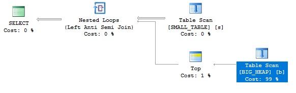
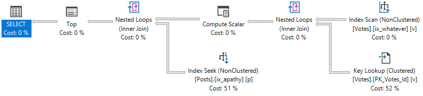
The plan doesn’t look so hot:
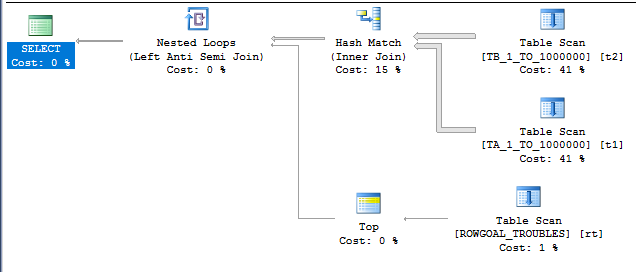
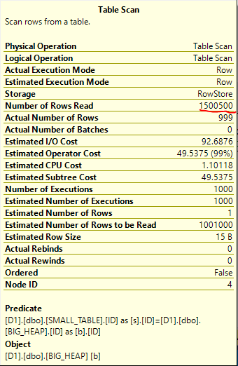
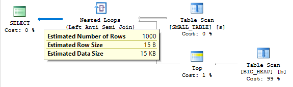
There are unmatched rows in the ROWGOAL_TROUBLES table, so we know that the scan on the inner side of the nested loop is going to read a lot of rows. The query took about 60 seconds to finish on my machine and read 499775000 rows from the ROWGOAL_TROUBLES table. Why did this plan seem attractive to SQL Server? The query optimizer thought that only 100 rows would be returned after the join of TA_1_TO_1000000 to TB_1_TO_1000000. The filters are perfectly correlated so 10000 rows will be returned in reality. With perfectly correlated filters we can expect a better estimate if we use simple containment:
SELECT *
FROM dbo.TA_1_TO_1000000 t1
INNER JOIN dbo.TB_1_TO_1000000 t2
	ON t1.UNIQUE_ID = t2.UNIQUE_ID
WHERE t1.MOD_FILTER = 1
AND t2.MOD_FILTER = 1
AND NOT EXISTS (
	SELECT 1
	FROM dbo.ROWGOAL_TROUBLES rt
	WHERE rt.UNIQUE_EVEN_ID = t1.UNIQUE_ID
)
OPTION (
MAXDOP 1,
USE HINT ('ASSUME_JOIN_PREDICATE_DEPENDS_ON_FILTERS')
);
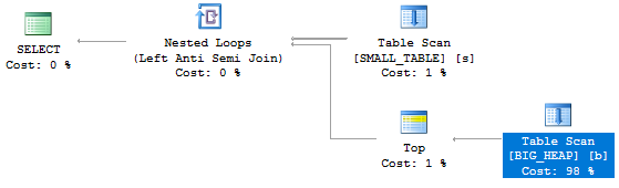
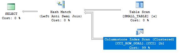
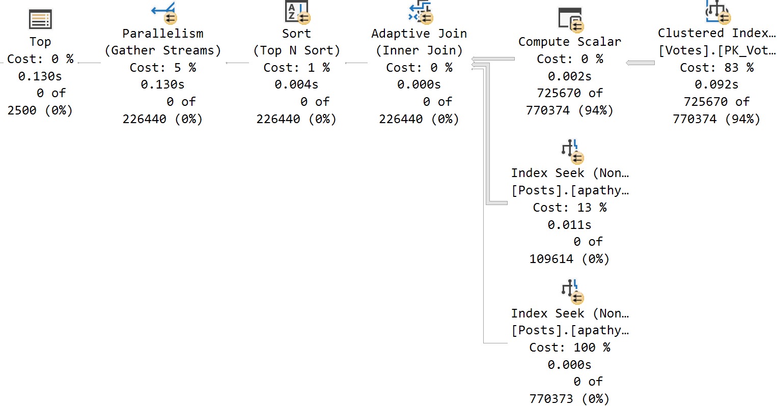
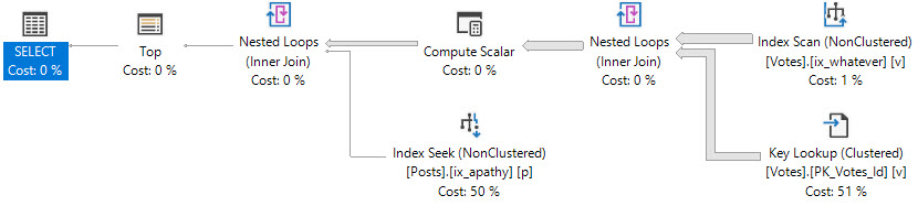
With a better estimate of 10000 rows comes a better query plan:

The query finishes in under a second on my machine.
Final Thoughts
Hopefully this blog post gives you a better understanding of the difference between base and simple containment. Read some of the other explanations out there if this wasn’t helpful. Containment is a tricky subject and you never know what it’ll take for it to make sense to you.
Thanks for reading!
Going Further
If this is the kind of SQL Server stuff you love learning about, you’ll love my training. I’m offering a 75% discount to my blog readers if you click from here. I’m also available for consulting if you just don’t have time for that and need to solve performance problems quickly.

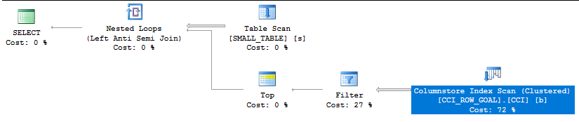
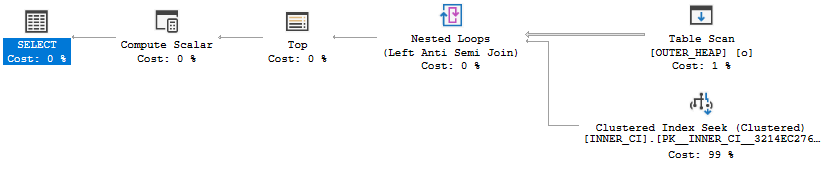 The plan has a total cost of 0.198516 optimizer units. If you know anything about row goals (this may be a good time for the reader to visit
 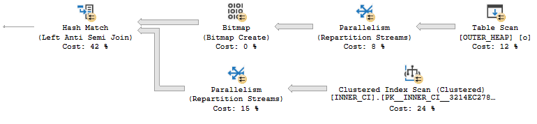 The new plan runs in
 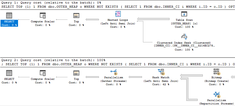 Something looks very wrong here. The loop join plan has a significantly lower cost than the hash join plan! In fact, the loop join plan has a total cost of 0.0167621 optimizer units. Why would disabling row goals for such a plan cause a decrease in total query cost?I uploaded the estimated plans
 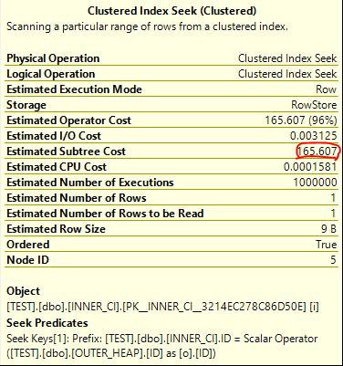 It's an exact match. The total cost of the query is 172.727 optimizer units, which is significantly more than the price tag of 19.9924 units for the hash join plan.
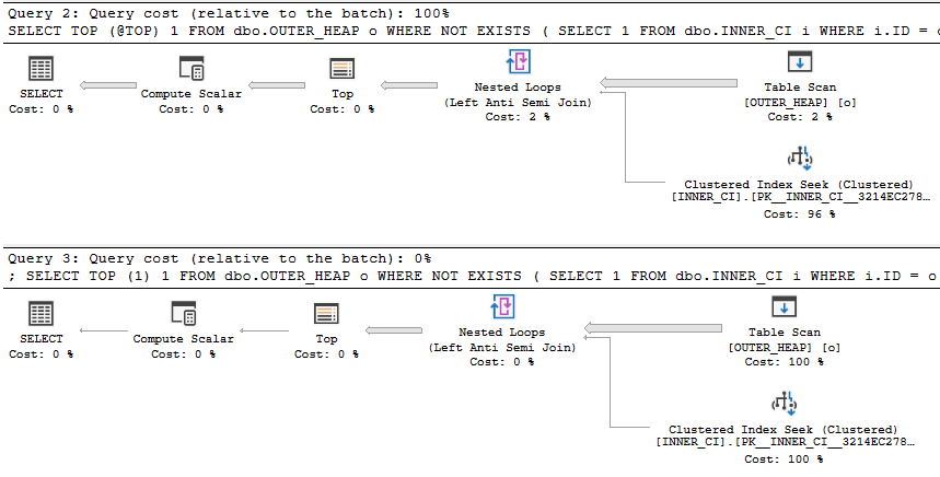 I also uploaded the estimated plans